Resampling the Efficient Frontier: An Illustration During the Codiv-19 Pandemic

Overview

A well-known problem with mean-variance portfolio optimization is that it is subject to instability: small changes in the inputs lead to large differences in the optimal portfolios. Since estimates of the required parameters (particularly the expected returns) using historical returns are extremely noisy, this results in unstable portfolios that would required frequent rebalancing. Another issue with this type of “blind” optimization is that, if an asset has much higher average returns over the sample period used to estimate the parameters, the optimal portfolios will tend to concentrate heavily on this asset, resulting in undiversified portfolios.

In this article, I illustrate this instability over a particularly volatile period, the Covid-19 crisis. I estimate the efficient frontier for a set of ETFs that represent different asset classes in the periods before and after the Covid crisis, showing that, not only does the frontier changes dramatically, but the “efficient” portfolios are heavily concentrated on just a few assets that happened to have better risk-adjusted performance during the estimation period.

Then, I apply a method that has been proposed to deal with these problems: resampling. The idea is to obtain many samples from the distribution of the returns of the assets, estimating the frontier in each of them, and averaging the resulting portfolio weights to create a resampled efficient frontier. This has the effect of reducing extreme concentrations and producing a more robust efficient frontier. I do this using two approaches: 1. assuming assets are normally distributed, and 2. using a simple bootstrap, drawing random samples with replacement from the history of past returns,

This illustration relies on the quantmodpackage to download assets returns, and the PortfolioAnalytics package for portfolio optimization. The focus on this article is on the illustration of the concepts; I’m sure there are many ways to optimize the code.

Setting the stage I consider a set of ETFs that represent different asset classes, including:

U.S. investment-grade bonds (BND)

International investment-grade bonds (IAGG)

High-yield bonds (GHYG)

U.S. equities (VTI)

Developed equities (VXUS)

Emerging market equities (VWO)

Commodities (GSG)

REITs (USRT).

I start by loading the required packages and downloading the data with the getSymbols function from the quantmod package. I use the viridis library for better-looking color palettes.

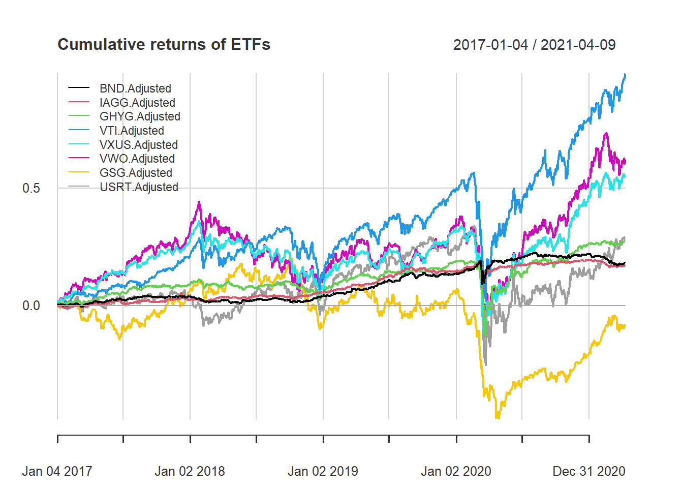
The commands below clear the workspace, load the required libraries, and download the prices of the ETFs. I then merge the adjusted prices into an xts object called prices.data. This makes it very straightforward to select specific date ranges. I use the CalculateReturns and chart.CumReturns functions from the PerformanceAnalytics package to easily obtain the returns of all assets and plot their cumulative returns.

 # Clear console
    shell("cls")

    # Clear environment
    rm(list = ls())

    # Load libraries
    library(PortfolioAnalytics)
    library(PerformanceAnalytics)
    library(quantmod)
    library(viridis)
    library(MASS)

    # Create an object with asset names
    asset_names <- c("BND", "IAGG", "GHYG", "VTI", "VXUS", "VWO", "GSG", "USRT")

    # Download data
    from.date <- as.Date("01/01/17", format="%m/%d/%y")
    options("getSymbols.warning4.0"=FALSE)
    getSymbols(asset_names, from = from.date)

    # Merge adjusted prices of all ETFs
    prices.data <- merge.xts(BND[,6], IAGG[,6], GHYG[,6], VTI[,6], VXUS[,6], VWO[,6], GSG[,6], USRT[,6])
    
    # Calculate returns of all ETFs
    returns.data <- CalculateReturns(prices.data)
    returns.data <- na.omit(returns.data)

    # Visualize cumulative returns
    chart.CumReturns(returns.data, main = "Cumulative returns of ETFs", legend.loc = "topleft")

Estimating the Effficient Frontier

I initially estimate the efficient frontier using three different samples (full sample, pre-covid, and post-covid). To make things easier, I create a wrapper function that estimates the efficient frontier for a given set of returns using functions from the PortfolioAnalytics package. The function takes as inputs a matrix of returns (R) and the number of portfolios along the efficient frontier (nPorts). The outputs include a data frame with the expected returns and volatilities of the portfolios along the efficient frontier, as well as the corresponding portfolio weights. In this example, all portfolios are long-only and fully-invested.

In principle, we could have used the Create.EfficientFrontier function, however it doesn’t always return the same number of portfolios.

 efficientFrontier.fn <- function(R, nPorts){

  # Expected returns and covariance matrix
  meanReturns <- colMeans(R)
  covMat <- cov(R)
  stdDevs <- sqrt(diag(covMat))
  
  # create a portfolio
  port <- portfolio.spec(assets = colnames(returns.data))
  
  # Adding a "box" constraint that weights should be between 0 and 1
  port <- add.constraint(port, type = "box", min = 0, max = 1)
  
  # Adding a leverage constraint for a fully-invested portfolio
  port <- add.constraint(portfolio = port, type = "full_investment")
  
  # Find the minimum-variance portfolio
  mvp.port <- add.objective(port, type = "risk", name = "var")
  mvp.opt <- optimize.portfolio(R, mvp.port, optimize_method = "ROI")
  
  # Find minimum and maximum expected returns, and define a grid with nPorts portfolios
  minret <- mvp.opt$weights %*% meanReturns
  maxret <- max(colMeans(R))
  target.returns <- seq(minret, maxret, length.out = nPorts)
  
  #Now that we have the minimum variance as well as the maximum return portfolios, we can build out the efficient frontier. 
  eff.frontier.return <- double(length(target.returns))
  eff.frontier.risk <- double(length(target.returns))
  eff.frontier.weights <- mat.or.vec(nr = length(target.returns), nc = ncol(returns.data))
  colnames(eff.frontier.weights) <- colnames(returns.data)
  
  for (i in 1:length(target.returns)) {
    eff.port <- add.constraint(port, type = "return", name = "mean", return_target = target.returns[i])
    eff.port <- add.objective(eff.port, type = "risk", name = "var")
    eff.port <- optimize.portfolio(R, eff.port, optimize_method = "ROI")
    eff.frontier.risk[i] <- sqrt(t(eff.port$weights) %*% covMat %*% eff.port$weights)
    eff.frontier.return[i] <- eff.port$weights %*% meanReturns
    eff.frontier.weights[i,] <- t(eff.port$weights)
    #print(paste(round(i / length(target.returns) * 100, 0), "% done..."))
  }
  
  # save everything as a list
  
  # efficient frontier
  eff.frontier <- as.data.frame(cbind(eff.frontier.risk, eff.frontier.return))
  names(eff.frontier) <- c("Risk", "Return")
  
  # add the weights
  out <- list(eff.frontier, eff.frontier.weights)
  names(out) <- c("EfficientFrontier", "Weights")
  return(out)
}
#end function

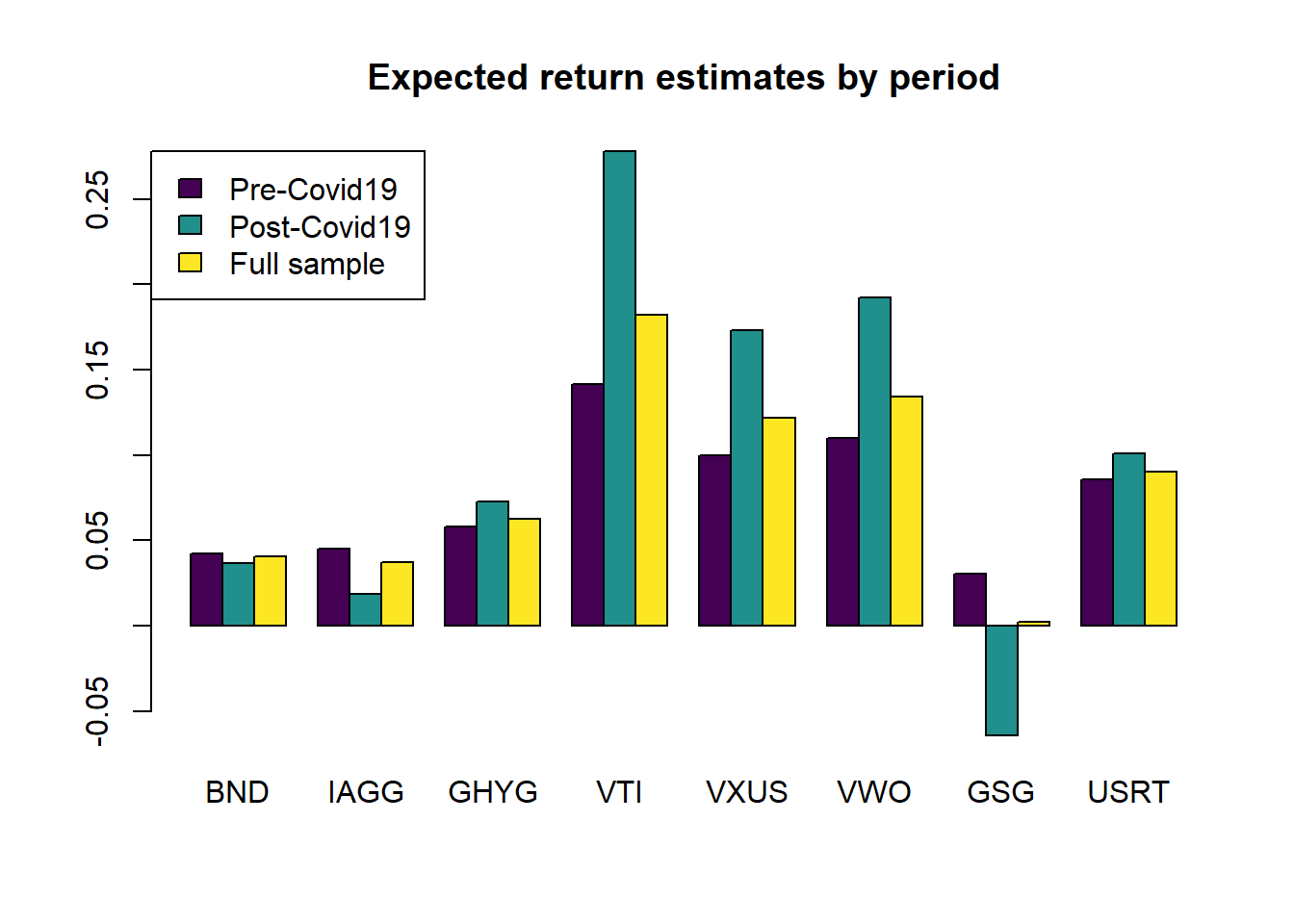
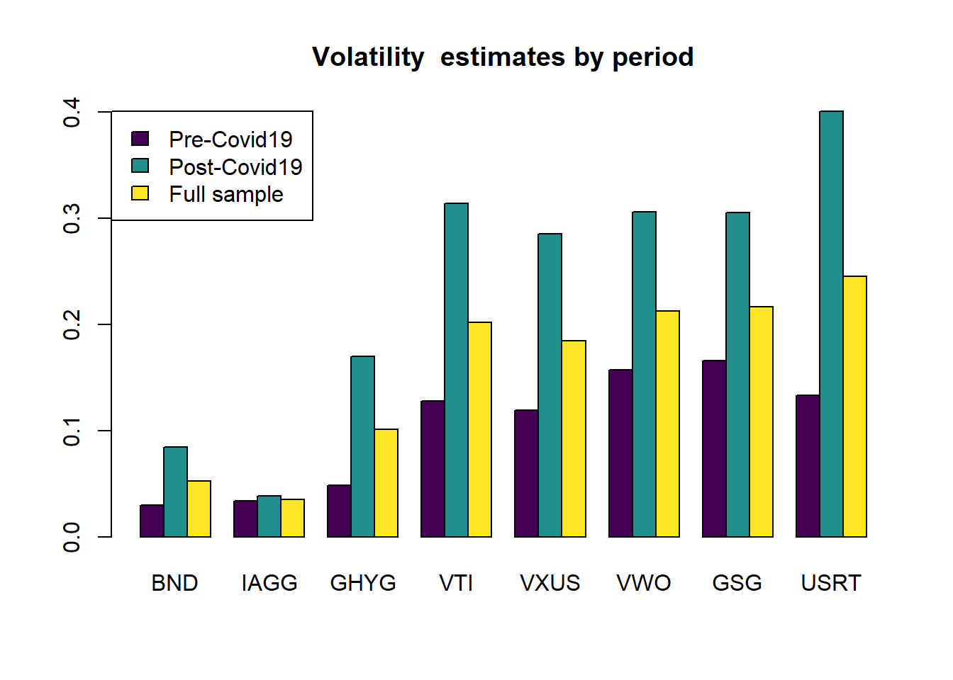
With the above function, it is straightforward to estimate the efficient frontier using any arbitrary sample of returns. I first create objects that identify the dates for each period. I consider as the starting date of the pandemic the beginning of 2020. I also show the expected returns and annualized volatilities in each period. It is clear that, while volatilities are much higher in the post-covid period across the board, the average returns for equities is actually higher in the post-covid period.

# indices of each sample 
full.sample   <-  index(returns.data) <= index(returns.data[nrow(returns.data)]) 
pre.covid19   <- index(returns.data) <=  as.Date("12/31/19", format = "%m/%d/%y")
post.covid19  <- index(returns.data)  >  as.Date("12/31/19", format = "%m/%d/%y")

# calculate average returns and volatilities in each period and plot them
mu_periods <- 252 * rbind(colMeans(returns.data[pre.covid19, ]), colMeans(returns.data[post.covid19, ]), colMeans(returns.data[full.sample, ]))
sd_periods  <- sqrt(252)* rbind (apply(returns.data[pre.covid19, ], 2, sd), apply(returns.data[post.covid19, ], 2, sd), ... =  apply(returns.data[full.sample, ], 2, sd))
rownames(mu_periods) <- c("Pre-Covid19", "Post-Covid19", "Full sample")
rownames(sd_periods) <- c("Pre-Covid19", "Post-Covid19", "Full sample")

# shorter names for bar plot
colnames(mu_periods) = asset_names
colnames(sd_periods) = asset_names

barplot(mu_periods, beside = TRUE, legend.text = TRUE,  col = viridis(3), 
        args.legend = list(x = "topleft"), 
        main = "Expected return estimates by period")

barplot(sd_periods, beside = TRUE, legend.text = TRUE,  col = viridis(3), 
        args.legend = list(x = "topleft"), 
        main = "Volatility  estimates by period")

Next, I use the efficientFrontier.fn function to obtain the different efficient frontiers. I use 60 portfolios, which is more than enough to provide a smooth representation of the frontier.

# estimating the efficient frontiers
num.ports <- 60

# Call our function to store the efficient frontier and weights for each sample
eff.frontier.full.sample   <-  efficientFrontier.fn(R = returns.data[full.sample, ],  nPorts = num.ports)
eff.frontier.pre.covid19   <-  efficientFrontier.fn(R = returns.data[pre.covid19, ],  nPorts = num.ports)
eff.frontier.post.covid19  <-  efficientFrontier.fn(R = returns.data[post.covid19, ], nPorts = num.ports)
  
# plot the efficient frontiers
par(mfrow = c(1,1))
plot(eff.frontier.full.sample$EfficientFrontier$Risk*sqrt(252), 
     eff.frontier.full.sample$EfficientFrontier$Return*252, 
     type = "l", col = "black",  ylim = c(0,0.3), xlim = c(0,0.4), 
     lwd = 2, xlab = "Risk", ylab = "Return")
par(new=TRUE)
plot(eff.frontier.pre.covid19$EfficientFrontier$Risk*sqrt(252), 
     eff.frontier.pre.covid19$EfficientFrontier$Return*252, 
     type = "l", col = "blue", ylim = c(0,0.3), xlim = c(0,0.4),
     lwd = 2, xlab = "Risk", ylab = "Return")
par(new=TRUE)
plot(eff.frontier.post.covid19$EfficientFrontier$Risk*sqrt(252),
     eff.frontier.post.covid19$EfficientFrontier$Return*252, 
     type = "l", col = "red", ylim = c(0,0.3), xlim = c(0,0.4),
     lwd = 2, xlab = "Risk", ylab = "Return")
legend(x = "bottomright", c("Full sample", "Pre-Covid19", "Post-Covid19"), 
       lty=c(1,1,1), lwd=c(2,2,2), col = c("black","blue","red"))
title("Comparison of efficient frontiers")

There is quite a large degree of instability in the efficient frontiers. The pre-covid efficient frontier is much “shorter”, reflecting a much narrower range for the risk estimates, and is located above the others in its range of volatilities. The post-covid efficient frontier extends much further to the right, due to the much higher volatilities, as well as the higher expected returns of equities.

Next, we inspect the weights along the efficient frontiers.

par(mfrow = c(3,1))
barplot(t(eff.frontier.full.sample$Weights),  col = viridis(ncol(returns.data)), 
        legend.text = asset_names, xlab = "Risk", ylab = "Weight", 
        names.arg = round(sqrt(252)*eff.frontier.full.sample$EfficientFrontier$Risk,2))
title("Efficient frontier weights - Full sample")
barplot(t(eff.frontier.pre.covid19$Weights),  col = viridis(ncol(returns.data)), 
        legend.text = asset_names, xlab = "Risk", ylab = "Weight", 
        names.arg = round(sqrt(252)*eff.frontier.pre.covid19$EfficientFrontier$Risk,2))
title("Efficient frontier weights - Pre-Covid19")
barplot(t(eff.frontier.post.covid19$Weights),  col = viridis(ncol(returns.data)), 
        legend.text = asset_names, xlab = "Risk", ylab = "Weight", 
        names.arg = round(sqrt(252)*eff.frontier.post.covid19$EfficientFrontier$Risk,2))
title("Efficient frontier weights - Post-Covid19")

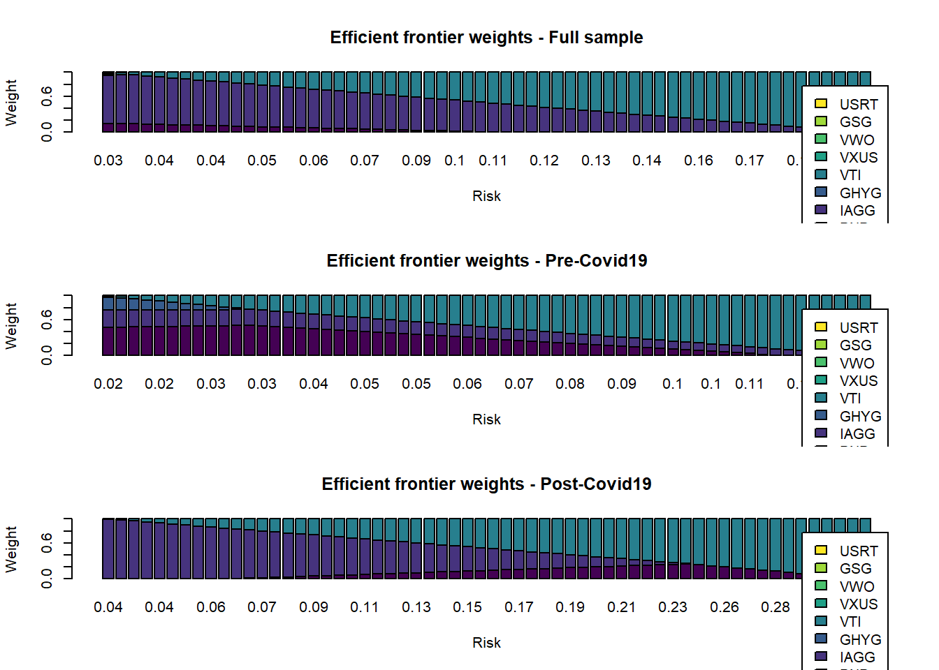
The composition of the efficient portfolios changes quite significantly depending on the sample period. It’s also evident that the efficient portfolios are not well diversified and are dominated by 2-3 assets. This is a well-known characteristic of Markowitz-style portfolio optimization. Practitioners usually add constraints on the range of weights to avoid this. We will now see a different approach using resampling.

Resampling the Efficient Frontier

We have seen previously that the efficient frontier is highly sensitive to the inputs, and usually is composed of portfolios that are not well diversified. Now, we will use a resampling technique to see if we can obtain more stable, more diversified efficient frontiers. Since we already have a function that produces the entire frontier, it is straightforward to use if for resampling. We will generate samples using two methods: MCMC simulation with a multivariate normal distribution, and historical simulation using actual returns. We will then average the weights obtained over the different sample, and build the resampled efficient frontiers using these weights.

I start by setting the number of samples to be drawn, and creating objects to store the results.

# number of samples
num.samples <- 200                    
# number of portfolios in efficient frontier
num.ports <- 60
# number of days to sample in each run - I used two years of daily returns
sample.size <- 252*2                   
# total number of days 
total.days <- nrow(returns.data)       
# create objects to store the resampled frontiers and weights
resampled.frontiers.Gaussian <- list()
resampled.weights.Gaussian <- mat.or.vec(nr = num.ports, nc = ncol(returns.data))
colnames(resampled.weights.Gaussian) <- colnames(returns.data)
resampled.frontiers.historical <- list()
resampled.weights.historical <- mat.or.vec(nr = num.ports, nc = ncol(returns.data))
colnames(resampled.weights.historical) <- colnames(returns.data)

# inputs for Gaussian simulation
expected.returns <- colMeans(returns.data)
cov.mat <- cov(returns.data)
stdDevs <- sqrt(diag(cov.mat))

Next, I simulate returns from the assets using the Gaussian and historical approaches. For each of these generated samples, I re-estimate the efficient frontier and store the results. This can take a while depending on the number of samples and portfolios in the efficient frontier. Of course, this could be easily parallelized.

# loop to generate samples and calculate efficient frontiers
for (i in 1:num.samples)
{
    # Resampling from a Gaussian distribution 
    sim.returns <- mvrnorm(sample.size, mu = expected.returns, Sigma = cov.mat)
    # transform to xts object to use with PortfolioAnalytics package
    sim.returns <-  xts(sim.returns, 
                        order.by = seq(as.Date("2000-01-01"), length.out=nrow(sim.returns), by = "day"), 
                        sim.returns)
    resampled.frontiers.Gaussian[[i]] <- efficientFrontier.fn(sim.returns, nPorts = num.ports)
    resampled.weights.Gaussian <- resampled.weights.Gaussian + resampled.frontiers.Gaussian[[i]]$Weights
    
    # Resampling using randomly drawn historical returns
    sample.inds <- sample(total.days, sample.size, replace = FALSE)
    resampled.frontiers.historical[[i]] <- efficientFrontier.fn(returns.data[sample.inds,], nPorts = num.ports)
    resampled.weights.historical <- resampled.weights.historical + resampled.frontiers.historical[[i]]$Weights
}
  
# calculate the average weights
resampled.weights.Gaussian <- resampled.weights.Gaussian/num.samples
resampled.weights.historical <- resampled.weights.historical/num.samples

# if there are NAs, it means at least one optimization failed. Remove these. 
resampled.weights.Gaussian <- resampled.weights.Gaussian[!is.na(rowSums(resampled.weights.Gaussian)),]
resampled.weights.historical <- resampled.weights.historical[!is.na(rowSums(resampled.weights.historical)),]

# calculate the risk and expected returns using the average resampled weights
resampled.risks.Gaussian <- double(nrow(resampled.weights.Gaussian))
resampled.returns.Gaussian <- double(nrow(resampled.weights.Gaussian))
resampled.risks.historical <- double(nrow(resampled.weights.historical))
resampled.returns.historical <- double(nrow(resampled.weights.historical))

# expected returns and risks using average weights from resampling
for (i in 1:nrow(resampled.weights.Gaussian))
{
  resampled.risks.Gaussian[i] <- sqrt(t(resampled.weights.Gaussian[i,])%*%cov.mat%*%resampled.weights.Gaussian[i,])
  resampled.returns.Gaussian[i] <- t(resampled.weights.Gaussian[i,])%*%expected.returns
}

for (i in 1:nrow(resampled.weights.historical))
{
  resampled.risks.historical[i] <- sqrt(t(resampled.weights.historical[i,])%*%cov.mat%*%resampled.weights.historical[i,])
  resampled.returns.historical[i] <- t(resampled.weights.historical[i,])%*%expected.returns
}

Finally, I compare the efficient frontier using the full sample, and the two resampled frontiers. For reference, I also include the base assets using their full-sample parameter estimates.

# plot the base assets and the efficient frontier using the whole sample
par(mfrow = c(1,1))
plot(eff.frontier.full.sample$EfficientFrontier$Risk*sqrt(252),
     eff.frontier.full.sample$EfficientFrontier$Return*252, 
     type = "l", col = "black",  ylim = c(-0.05, 0.3), xlim = c(0,0.3), 
     lwd = 2, xlab="Risk",ylab="Return")
par(new=TRUE)
plot(sd_periods["Full sample", ], mu_periods["Full sample", ],
     pch = 16, main = "Eficient frontier: full sample vs resampled",
     col = "blue", ylim = c(-0.05, 0.3), xlim = c(0,0.3), xlab = "Risk", ylab = "Return")
text(sd_periods["Full sample", ], mu_periods["Full sample", ], labels = asset_names, pos=1)


# plot resampled efficient frontiers
par(new = TRUE)
plot(resampled.risks.Gaussian*sqrt(252), resampled.returns.Gaussian*252, 
     type = "l", col = "green",  c(-0.05, 0.3), xlim = c(0,0.3), 
     lwd = 2, xlab = "Risk", ylab = "Return")
par(new=TRUE)
plot(resampled.risks.historical*sqrt(252), resampled.returns.historical*252, 
     type = "l", col = "red", ylim = c(-0.05, 0.3), xlim = c(0,0.3), 
     lwd = 2, xlab = "Risk", ylab = "Return")
legend(x = "topleft", c("Full sample", "Resampled Gaussian", "Resampled Historical"),
       lty = c(1,1,1), lwd = c(2,2,2), col = c("black","green","red"))

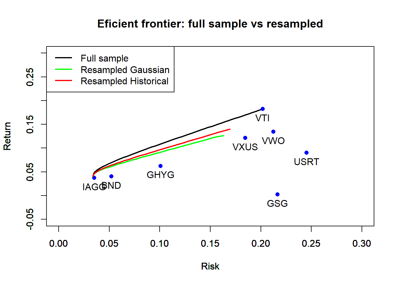
The two resampled frontiers are very similar and they both lie below the efficient frontier obtained using the full sample. This is not unexpected, because the frontier using the full sample has extreme weights on the assets with highest expected return estimates, whereas in the resampled frontiers, this effect will be averaged out.

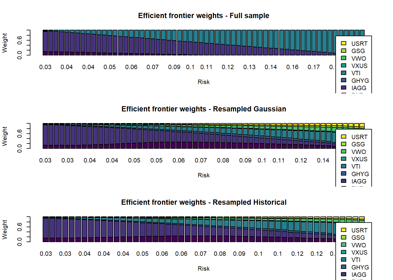
Resampling and Portfolio Diversification

Does resampling help in terms of increasing the diversification along the efficient frontier? Indeed, resampling dramatically improves the diversification of the portfolios in the efficient frontier. When the full sample is used, the portfolios are extremely concentrated in bonds (BND/IAGG) for low risk portfolios and in U.S. equities (VTI) for high risk portfolios. The resampled efficient frontiers have a much better diversification and typically invest in all asset classes. This example suggest that resampling is an effective way to obtain more robust estimates of efficient portfolios.

# inspect weights along full-sample and resampled efficient frontiers
par(mfrow = c(3,1))
barplot(t(eff.frontier.full.sample$Weights),  
        col = viridis(ncol(returns.data)), 
        legend.text = asset_names, xlab = "Risk", ylab = "Weight", 
        names.arg = round(sqrt(252)*eff.frontier.full.sample$EfficientFrontier$Risk,2))
title("Efficient frontier weights - Full sample")

barplot(t(resampled.weights.Gaussian),  col = viridis(ncol(returns.data)), 
        legend.text = asset_names, xlab = "Risk", ylab = "Weight", 
        names.arg = round(sqrt(252)*resampled.risks.Gaussian,2))
title("Efficient frontier weights - Resampled Gaussian")

barplot(t(resampled.weights.historical),  col = viridis(ncol(returns.data)), 
        legend.text = asset_names, xlab = "Risk", ylab = "Weight", 
        names.arg = round(sqrt(252)*resampled.risks.historical,2))
title("Efficient frontier weights - Resampled Historical")

Concluding Remarks

This article illustrates two issues associated with mean-variance portfolio optimization. First, the portfolios tend to be extremely concentrated in only a few assets. Second, the efficient frontier is unstable when the sample period used to estimate the parameters changes, which is shown by comparing the efficient frontiers before and after the start of the Covid-19 crisis. A resampling method, which has been proposed to produce more robust estimates of the efficient frontier, is illustrated using simulations from a normal distribution or from historical returns. The resampled efficient frontier is obtained by averaging the weights obtained with each simulated sample. The resampled frontiers obtained with the two resampling methods in this example are similar, and much more diversified than the efficient frontier obtained using the full sample.