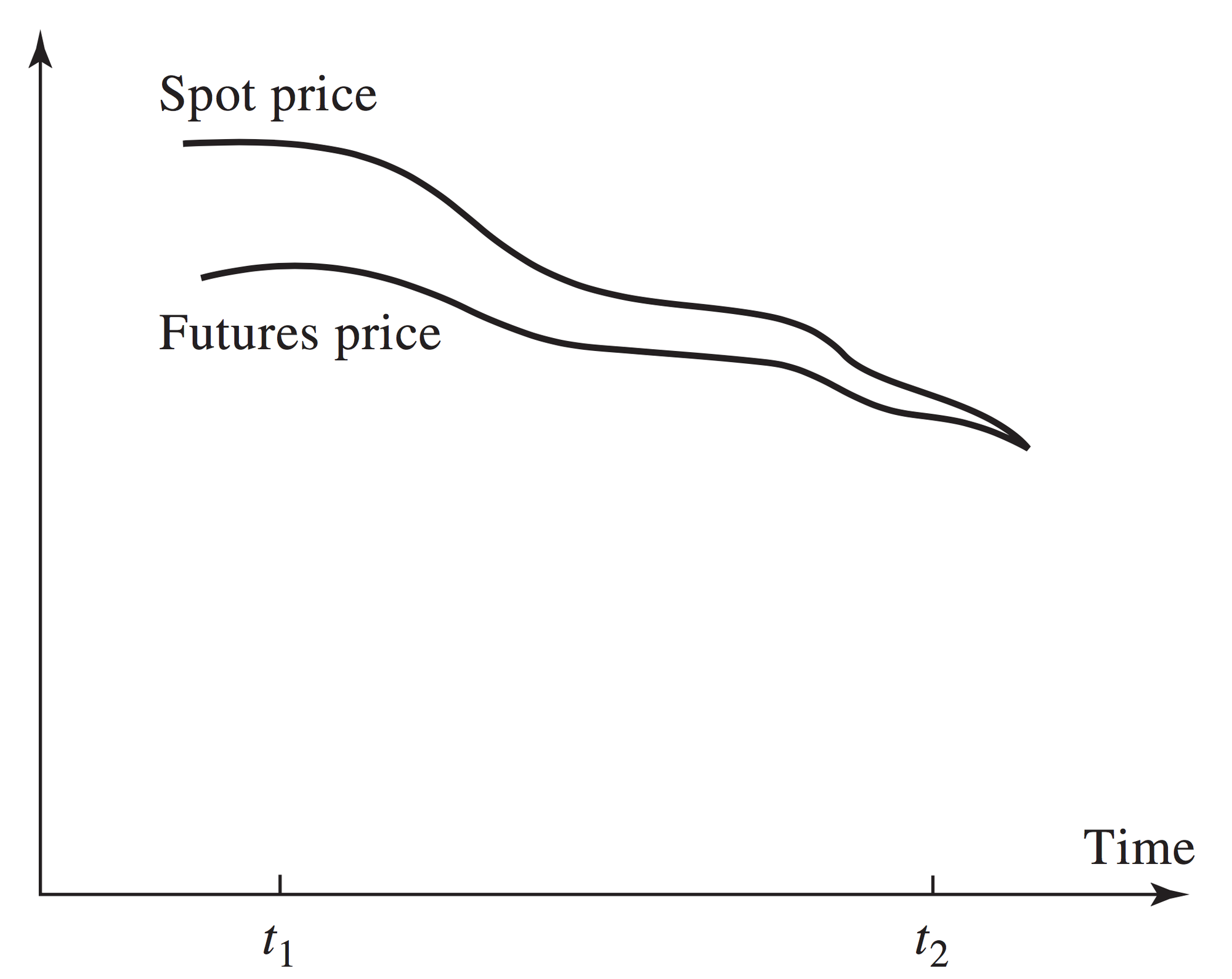
Hedge Ratio
Introduction
This is a series of short articles to discuss the tools to manage risk in the commodity markets using R. My goal is to show how can we optimize the hedging strategy using commodities contracts - futures and options.
Load some packages.
library(tidyverse)
library(quantmod)
library(zoo)
library(ggplot2)
library(Quandl)
library(lubridate)
library(ggthemes)
library(reshape)
library(riskR)
library(stargazer)
library(tinytex)
Forward-Spot relationship
-The relationship between the forward and the spot price, assuming no-arbitrage, can be describe as follows Geman (2005): \begin{align} f ^T (t) = S(t)e^{(r-y)(T-t)} \end{align} where $r$ is the continuously compound interest rate at instant t and maturity $T$, and $y$ is the convenience yield.
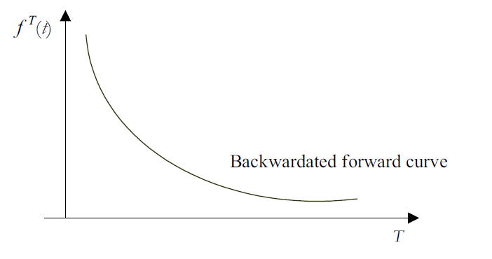
We call backwardation when $(r-y) < 0$, the forward curve is a decreasing function of maturity.
![]()
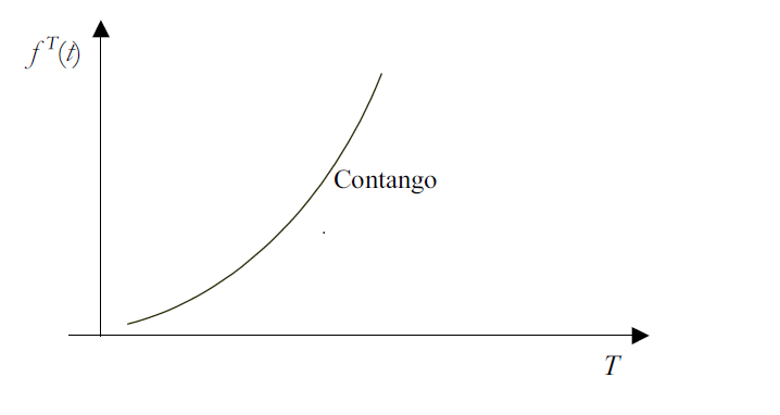
The contango sitaution is when $(r-y) > 0$, the forward curve is an increasing function of maturity.
![]()
Extract the Soybean prices from Quandl.
soy = Quandl("TFGRAIN/SOYBEANS")
soy_f = soy  %>%
  mutate(soy, Futures = soy$`Cash Price`-soy$Basis)
dd= soy_f[,c(1:2, 6)]
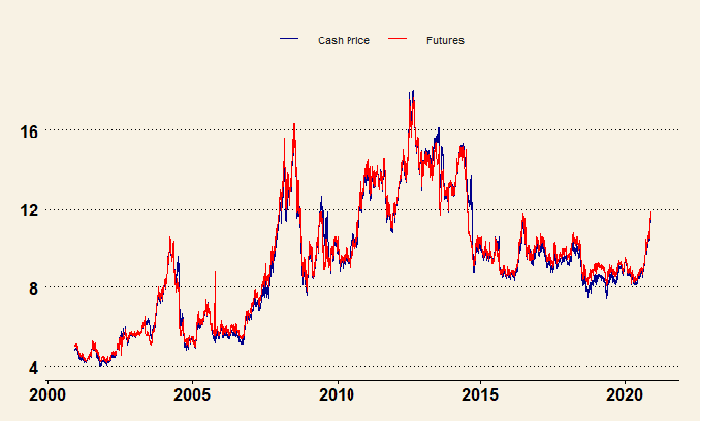
Spread Futures vs Spot price.
Let’s assume the Basis as only the spread between Spot and Future price.
Supposing you want to hedge a Cash Price position (Spot) with a Future contract (F) in the Chicago Mercantile Exchange (CME).

Build ggplot.
dd1= melt(dd,id=c("Date"))

dd1 %>%
  ggplot(aes(x=Date, y=value,color=variable))+geom_line()+
  theme_wsj()+
   xlab(" ")+ylab(" ")+
   scale_colour_manual("",
                      breaks = c("Cash Price", "Futures"),
                      values = c("Cash Price"="darkblue", "Futures"="red"))+
  theme(legend.text = element_text(size = 8, colour = "grey10"))

Hedge Ratio.
- The hedge ratio is a measure that compares a financial asset to a hedging instrument. The measurement indicates the risk of a shift in the hedging instrument (Lien,2016). \begin{align} H^* = \rho \frac{\sigma_S}{\sigma_F} \end{align}
\begin{align} H_{mv}= \frac{Cov(\Delta S_t, \Delta f_t)}{Var(\Delta f_t)} \end{align}
- In the commodity markets is common to use Futures contracts to hedge the Spot price. If a producers/exporters want to hedge their production, for example, then they would sell Futures contracts; if a buyers/importers want to hedge their position in the futures markets, then they would buy futures contracts. In this sense, the hedge ratio indicates the level of risk a producer/exporter are exposed.
Time series - zoo.
data.z = zoo(dd[,-1], as.Date(dd[,1], format="%Y/%m/%d"))
S = data.z[,"Cash Price",drop=FALSE]
F = data.z[,"Futures",drop=FALSE]
# Estimating the returns
lS= diff(log(S))
lF=diff(log(F))
# Hedge Ratio
H = cov(lS,lF)/cov(lF)
stargazer(H, type = "text", title="Hedge Ratio", rownames = FALSE,
          colnames = FALSE)
Now suppose a company/importer knows that it will buy 1,000,000 of soybeans in one month. The soybean futures contract unit is 5,000/bushels. So, the number a futures contract (long position) the company will buy is…
N = H*(1000000/5000) #buy 190 futures contracts
stargazer(N, type = "text", title="N of Contracts", rownames = FALSE,
          colnames = FALSE)
Risk Metrics. Estimating optimal hedging ratios based on risk measures (see, Chan (2019)).
- The risk manager’s role is to mitigate the volatility by hedging the underlying asset or avoiding the deviation from the expected value.
- There are a few risk metrics to measure the uncertainty in the futures contracts. Chan (2019) created a package that computes 26 financial risk measures. Thus, we applied the function to our example (soybean hedging).
We use the Soybean Future contract (F) for hedging the Spot price (S).
rh = riskR::risk.hedge(lS,lF,alpha=c(0.05, 0.01), beta = 1, p=2)
stargazer(rh,type="text",font.size = 'tiny',
          no.space = TRUE, column.sep.width = '4pt', title="Risk Metrics")
Descriptions:
- Risk measures (Standard Deviation (StD)
- Value at Risk (VaR)
- Expected Loss (EL)
- Expected Loss Deviation (ELD)
- Expected Shortfall (ES)
- Shortfall Deviation Risk (SDR) Expectile Value at Risk (EVaR)
- Deviation Expectile Value at Risk (DEVaR)
- Entropic (ENT)
- Deviation Entropic (DENT)
- Maximum Loss (ML)
References
Chan, S., & Nadarajah, S. (2019). Risk: An R Package for Financial Risk Measures. Computational Economics, 53(4), 1337–1351. https://doi.org/10.1007/s10614-018-9806-9
Geman, H. (2005). Commodities and commodity derivatives. In J. W. & Sons (Ed.), Modeling and Pricing for Agriculturals, Metals and … (p. 419). John Wiley \& Sons.
Lien, D., Shrestha, K., & Wu, J. (2016). Quantile Estimation of Optimal Hedge Ratio. Journal of Futures Markets, 36(2), 194–214. https://doi.org/https://doi.org/10.1002/fut.21712
Please, cite this work:
Palazzi, Rafael (2022), “Hedge Ratio published at Open Code Community”, Mendeley Data, V1, doi: 10.17632/sccbtd2y29.1

