Overview

Crypto currencies have historically gone through extreme drawdowns. In this short post, we explore how the recent sell-off in crypto compares with the drawdowns observed historically. For the rest of this piece, we use the term “DD” to refer to drawdowns.

Load some packages.

rm(list = ls())
library(data.table)
library(quantmod)
library(rvest)
library(tidyverse)
library(PerformanceAnalytics)
library(ggplot2)
library(viridis)

Getting data from the largest crypto currencies

Most sources online use the use the crypto package to get historical data on cryptos. crypto, in turn scrapes data from coinmarketcap. However, changes in the way the data are represented in the site frequently break the package. Instead, we scrape the Yahoo Finance cryptocurrencies page to get the 100 largest coins. We remove empty values and stablecoins (Tether and USDC).

website <- read_html("https://finance.yahoo.com/cryptocurrencies/?count=100&offset=0")

coins <- website %>% 
  html_nodes("td a") %>% 
  html_text()

coins <- coins[coins != ""]

# remove stablecoins
coins <- coins[coins!="USDT-USD"]
coins <- coins[coins!="USDC-USD"]

Next, we get the data using getSymbols and create a single xts object with all the prices. we keep only coins that have a price history starting at least in 2018, replace missing values in the middle of the series with the last available ones, and then calculate the returns.

from.date <- as.Date("01/01/10", format="%m/%d/%y")
getSymbols(coins, from = from.date)

# merge all prices into a single xts object
coin_prices <- xts()
for (i in 1:length(coins)){
  coin_prices  <- merge.xts(coin_prices, get(coins[i])[,6])
}

colnames(coin_prices) <- gsub(".USD.Adjusted", "", colnames(coin_prices))

# find first available price
first_non_na <- function(x){
  return(min(which(!is.na(x))))
}

first_price_index <- apply(coin_prices, 2, first_non_na)

# keep only coins that have existed from at least 2017
keep_coins <- first_price_index <= min(which(index(coin_prices) >= "2018-01-01"))

(sum(keep_coins))

coin_prices <- coin_prices[, keep_coins]

# replace missing values with last value
coin_prices <- na.locf(coin_prices)

# calculate returns
coin_returns <- CalculateReturns(coin_prices)

Most crypto currencies reached their peaks recently. The graph below shows the the recent price history for Bitcoin, Ethereum, Binance Coin and, well, Doge:

par(mfrow = c(2,2))
plot(coin_prices$BTC["2021-04/"], main = "", 
     legend.loc = "topleft")
plot(coin_prices$ETH["2021-04/"], main = "",
     legend.loc = "topleft")
plot(coin_prices$BNB["2021-04/"], main = "", 
     legend.loc = "topleft")
plot(coin_prices$DOGE["2021-04/"], main = "",
     legend.loc = "topleft")

Bitcoin reached its all-time peak of 63503.46 on April 13, 2021 and was trading at $45275 on May 18, 2021, a ~29% correction. For Ethereum, the peak was 4168 on May 11, and the price is currently hovering around 3500, a 16% fall. Binance Coin dropped from a peak of 675 on May 3rd to about 524 (22% fall). Finally, DOGE reached a peak of 0.68 on May 7 and is currently trading at 0.49 (a ~27% correction). The values can be obtained with the code below (although this is not very efficient).

select_coins <- c("BTC", "ETH", "BNB", "DOGE")
max_inds <- apply(coin_prices[, select_coins], 2, which.max)

max_values <- coin_prices[max_inds,select_coins]
current_values <- coin_prices[nrow(coin_prices),select_coins]

rbind(max_values, current_values)

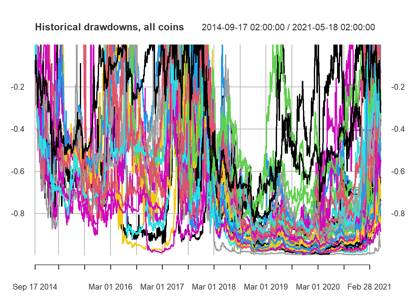
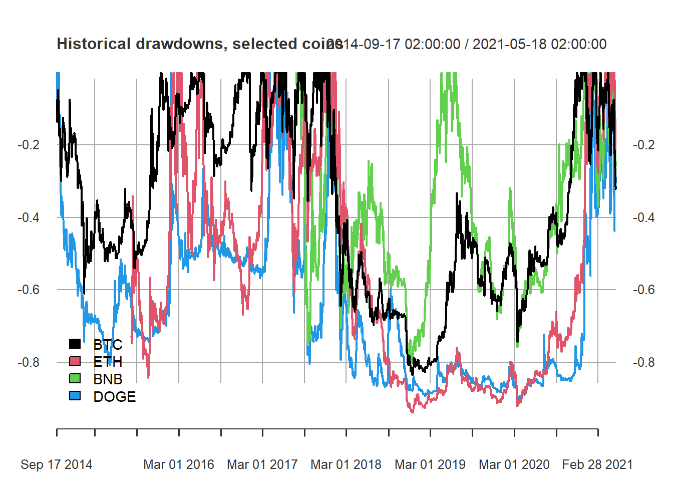
We can calculate the DDs for all coins using the code below. Although plotting all DDs in the same graph will make it hard to identify individual coins, it is interesting to show the pervasiveness of extreme DDs in crypto currencies. We also plot the historical DDs of the 4 selected coins. As expected, extreme DDs (80% to 90%+) are the norm in cryptoland.

# calculate drawdowns
DD <- Drawdowns(coin_returns)

plot(DD,
     main = "Historical drawdowns, all coins")

# plot the historical DDs of some coins (BTC, ETH, BNB, DOGE)
plot(DD[, select_coins],
     main = "Historical drawdowns, selected coins", 
     legend.loc = "bottomleft")

To provide some perspective, let’s compare the drawdowns of Bitcoin and the S&P 500.

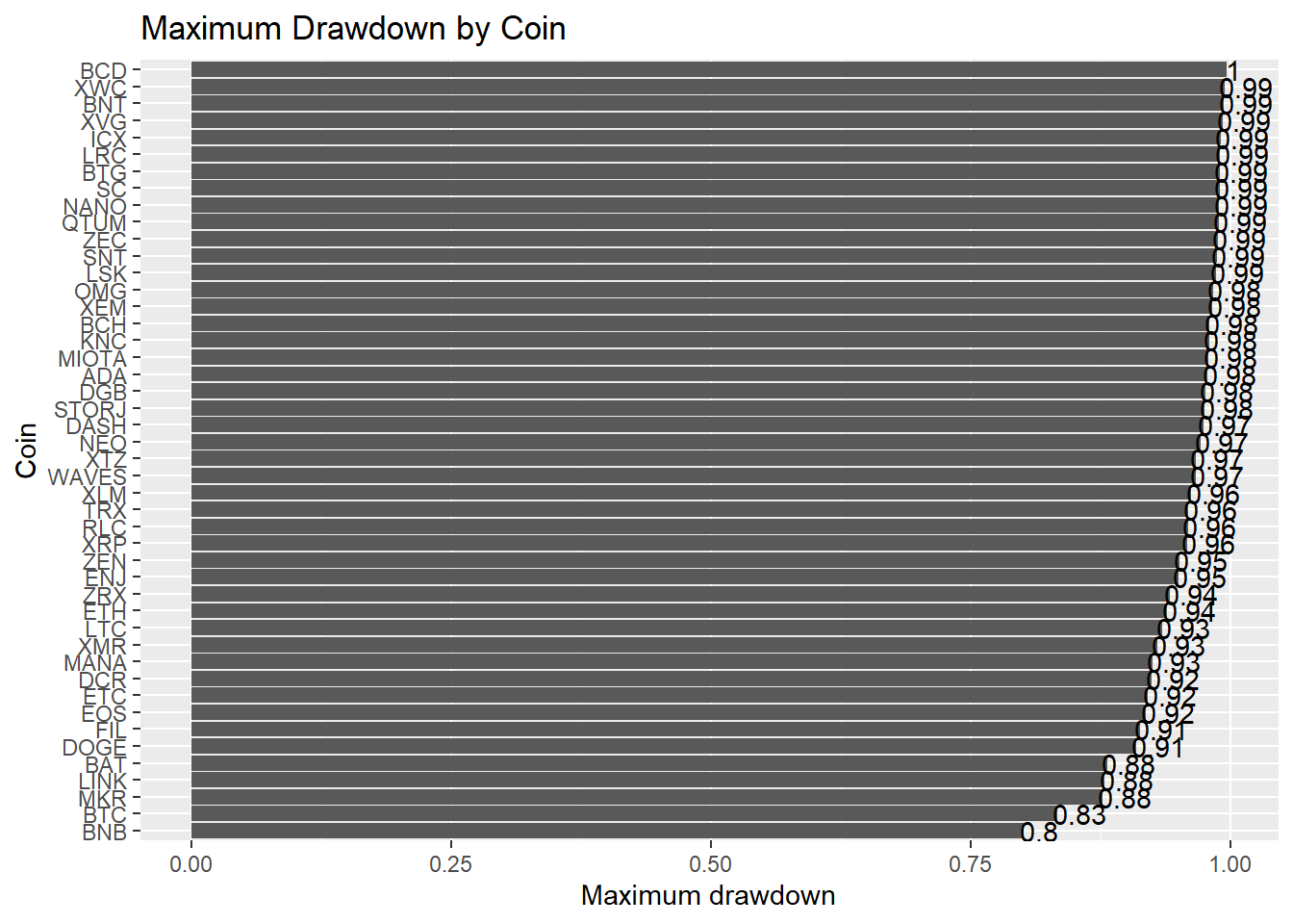
How does the current correction in crypto currencies compare to the maximum DDs observed historically? The code below gathers the maximum DDs and current DDs for all coins, and produces two bar plots:

# Max DD and Current DD by coin
DD_stats <- data.frame(Max.DD = -apply(coredata(DD), 2, min, na.rm = TRUE), 
                       Current.DD = -t(coredata(DD[nrow(DD),])))
DD_stats["Coin"] <- rownames(DD_stats)

# barplot of max DD by coin
p<- ggplot(DD_stats, aes(x = reorder(Coin, Max.DD), Coin, y=Max.DD)) + 
  geom_bar(stat = "identity") + geom_text(aes(label=round(Max.DD,2)), hjust=+0.1) + 
  coord_flip()
p + ggtitle("Maximum Drawdown by Coin") +
  ylab("Maximum drawdown") + xlab("Coin")

# barplot of current DD by coin
p<- ggplot(DD_stats, aes(x = reorder(Coin, Max.DD), Coin, y=Current.DD)) + 
  geom_bar(stat = "identity") + geom_text(aes(label=round(Current.DD,2)), hjust=+0.1) + 
  coord_flip()
p + ggtitle("Current Drawdown by Coin") +
  ylab("Current drawdown") + xlab("Coin")

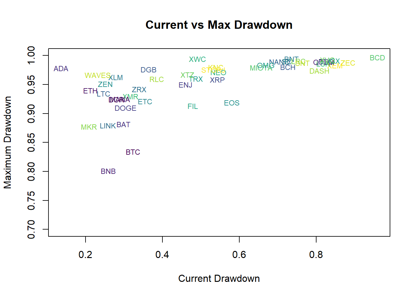
It’s clear that very high maximum DDs are common to almost all coins. In fact, no crypto currency in the list has a maximum DD lower than 80%. In contrast, there is a wide range for the current DDs. To visualize this, we plot the maximum vs current drawdown for all coins. For the largest and best-known cryptos (BTC, ETH, ADA, BNB and, well, DOGE), current DDs are relatively low relative to maximum drawdowns.

# plot current vs maximum drawdown
plot(DD_stats$Current.DD, DD_stats$Max.DD, type = "n", 
     main = "Current vs Max Drawdown",
     xlab = "Current Drawdown", 
     ylab = "Maximum Drawdown", 
     ylim = c(0.7,1))
text(DD_stats$Current.DD, DD_stats$Max.DD,
     labels = rownames(DD_stats), 
     cex = 0.75, font = 1, col = viridis(23))

Conclusion

Cryptocurrencies experience extreme levels of drawdown. In this short post, we calculate the drawdown of the largest cryptocurrencies, using historical data from 2017. No cryptocurrency in the list has a maximum drawdown lower than 80%. In contrast, the recent correction in cryptos seems relatively low, with the most popular (and largest) cryptocurrencies, like Bitcoin, Ethereum, Binance Coin, and, well, Doge.