Identifying turning points in aggregate economic series represents a topic of great practical and academic interest, at least since the seminal work of Burns and Mitchell (1946). How do we know if the economy is in a recession? How do we know when it has ended? Can we establish a chronology of recessions and expansions for a given economy?

To answer questions like these, one must rely on either a purely qualitative analysis (judgment of individuals) or a statistical method to identify turning points in a given time series. Of course, the latter may be (and probably should be) combined with qualitative assessments. Worldwide, one can observe formal organizations that date the business cycles in countries such as the U.S. (National Bureau of Economic Analysis - NBER), Euro Area (Centre for Economic Policy Research - CEPR), and Brazil (Brazilian Business Cycle Dating Committee - CODACE).

In this short note, we apply Harding and Pagan’s (2002) quarterly approximation to the Bry-Boschan (B.B.) algorithm (Bry and Boschan, 1971) to identify turning points at the Brazilian quarterly GDP seasonally adjusted series. As Colombo and Lazzari (2020) describe, the B.B. algorithm is a way of automatizing the cycle dating procedure according to the tradition of the NBER. In a nutshell, the method considers some rules imposed on the behavior of the series to classify peaks and troughs. A recession occurs from peak to trough, and an expansion occurs from trough to peak. First, a window is chosen to identify local maxima ($y_{t-k},…,y_{t-1}<y_{t}>y_{t+1},…,y_{t+k}$) and minima ($y_{t-k},…,y_{t-1}> y_{t}<y_{t+1},…,y_{t+k}$) in the reference series (parameter k). Second, a minimum period is required for the duration of a phase of the cycle (peak to trough or trough to peak - parameter p). Third, the algorithm also requires a parameter for the minimum duration of the complete cycle (peak to peak or trough to trough - parameter c). In our exercise, we follow Harding and Pagan (2002) and use k = 2, p = 2, and c = 5 quarters.

Furthermore, following Harding and Pagan (2002), we rely on the classical definition of cycle - the one that refers to the behavior of the level of a variable (as opposed to the growth or the growth rate of business cycles). Definitions of the business cycles can be found at OECD (2001). Besides being simple and straightforward, the B.B. algorithm almost replicates the chronology of recession and expansions compared with the NBER dating (Marcellino, 2006).

Now, we apply the referred methodology using Stata 15. One can apply the same procedure using other statistical software (e.g., package “BCDating” in R).

We start our exercise by downloading the quarterly Brazilian GDP at constant prices and seasonally adjusted from FRED (series I.D. = NAEXKP01BRQ652S) at Stata 15:

  import fred NAEXKP01BRQ652S, clear

After that, we set the data to time series' structure, using the FRED’s auto-generated time variable “daten”:

  tsset daten

Before proceeding to the analysis, one may want to divide the data (in R$) by 1,000,000,000, so we can interpret the numbers as Billions of Reais.

  replace NAEXKP01BRQ652S = NAEXKP01BRQ652S/1000000000

Now we can have a first taste of the dataset. We may analyze basic descriptive statistics:

  summ NAEXKP01BRQ652S  

Below I report the results from the summarize command. From 1996Q1 to 2020Q4, the average quarterly GDP of Brazil (in Brazilian Reais of 2000) was R$250.5 billion, ranging from 175.57 (1996Q1) to 312.52 (2019Q4).

Before using the B.B. algorithm, we transform the daily date variable into its quarterly counterpart and format it accordingly:

gen yq = qofd(daten)
format yq %tq

Now we proceed step-by-step to apply the B.B. algorithm for quarterly data as in Harding and Pagan (2002):

Step #1: Downloading the user-written SBBQ package

If not already installed, one should download the SBBQ package, written by Philippe Bracke (London School of Economics, U.K.):

ssc install sbbq

Step #2: Logarithmic transformation at the underlying series.

gen lnNAEXKP01BRQ652S = 100*ln(NAEXKP01BRQ652S)

Step #3: Applying the BB algorithm

sbbq lnNAEXKP01BRQ652S, w(2) p(2) cycle(5)

As we discussed before, we use 2, 2 and 5 quarters for the symmetric window, minimum phase duration, and minimum cycle duration, respectively.

Step #4: Transforming the result into a Recession Dummy (1 = rec, 0 = expansion)

After running the sbbq command, the package automatically creates a new variable in the dataset: “x_point”, where x is the name of the reference variable (lnNAEXKP01BRQ652S in our case). We might look at the local maxima (1) and minima (-1) identified by the algorithm using the following command (results on the Table below):

list yq lnNAEXKP01BRQ652S_point if inlist(lnNAEXKP01BRQ652S_point,1,-1)

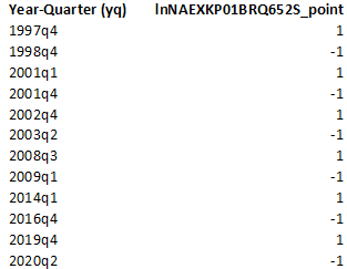
As we can see, there are six peaks and six troughs identified. However, before graphing the results, one must transform the x_point variable into a binary variable equal to one (if in a recessionary phase) or zero (otherwise). We do that by generating a variable called “gdp_rec”:

gen gdp_rec = 0
replace gdp_rec=1 if lnNAEXKP01BRQ652S_point[_n-1]==1
replace gdp_rec=1 if gdp_rec[_n-1]==1 & lnNAEXKP01BRQ652S_point[_n-1]!=-1 

Now we have a variable (gdp_rec) that equals one from the quarter immediately after an identified peak to a trough (i.e., a recession), and equals zero from trough to peak (i.e., an expansion) in the reference, underlying GDP series.

Before analyzing the results graphically, we label the variables so we can have pretty good looking figures:

label var NAEXKP01BRQ652S "Brazilian Quarterly GDP - Seasonally Adjusted"
label var gdp_rec "Economic Recessions in Brazil (CODACE)" 

Step #5: Graphical analysis

Now its time to analyze the results of the BB algorithm by comparing the recession dummy with the Brazilian Quarterly GDP:

twoway 	(bar gdp_rec yq if yq>=tq(1996q1), yaxis(1) yscale(log) ylabels(, nolabels) graphregion(color(white)) bgcolor(white) bcolor(gs14) cmissing(n) ytitle("")) ///
        (line NAEXKP01BRQ652S yq if yq>=tq(1996q1), yscale(log) color(navy) lwidth(0.5) yaxis(2) ylabels(, nolabels) ytitle("BRL Billion", axis(2))) , ///
        xtitle("") ///
        xla(#12, valuelabels ang(45)) ///
        legend(region(lcolor(white))) ///
        yline(0.5) ///
        graphregion(color(white)) bgcolor(white) plotregion(fcolor(white)) graphregion(fcolor(white)) legend(col(1))

The resulting Figure is the one presented below:

The shaded areas represent recession periods identified by the proposed algorithm. As expected, these periods coincide with falling GDP (i.e., negative real growth rates). We observe recessions in the following periods: 1998Q1-1998Q4, 2001Q2-2001Q4, 2003Q1-2003Q2, 2008Q4-2009Q1, 2014Q2-2016Q4, 2020Q1-2020Q2.

However, one question remains: how accurate is the chronology of recessions dated by the B.B. algorithm? One way to assess such accuracy is to compare it with the one released by the Brazilian Economic Cycle Dating Committee (CODACE). Using the last release from the committee, from June 29, 2020, we get the following picture:

The series analyzed by CODACE starts in 1980, thus being different from ours (beginning in 1996). Focusing on 1996 onwards (for comparison purposes), one will find that CODACE points out six recessions: around 1998-1999, 2001, 2003, 2008-2009, 2014-2016, and 2020. Those dates seem to coincide with ours! However, to check how much they overlap, we must take a closer look at both chronologies:

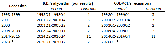
Wow, what a tremendous overlap! Except for the first recession (where our algorithm suggests the recession would have ended one quarter earlier), all else coincides. Moreover, our exercise reveals another important feature: we did not find any false positive (a situation where the algorithm indicates a recession not confirmed by the benchmark). Overall, our empirical exercise suggests that applying the B.B. algorithm on the Brazilian Quarterly GDP (seasonally adjusted) captures the chronology of economic recessions in a very accurate way compared to our benchmark (CODACE).

Such a good performance of the B.B. indicator is not a surprise. Colombo and Lazzari (2020) find the same evidence. Based on such an excellent performance of the algorithm, they apply the same procedure on the states' monthly index of economic activity (IBC-R from the Central Bank of Brazil) and find that the 2014-2016 great economic recession in Brazil was considerable heterogeneous across the Brazilian states (in terms of duration and magnitude). Their results might be replicated using the uploaded data in Colombo (2021).

References

• Bracke, P. (2012). SBBQ: Stata module to implement the Harding and Pagan (2002) business cycle dating algorithm.

• Bry, G., & Boschan, C. (1971). Programmed selection of cyclical turning points. In Cyclical analysis of time series: Selected procedures and computer programs (pp. 7-63). NBER.

• Economic Cycle Dating Committee – CODACE (2020). Announcement of the beginning of a recessionary phase in brazil in early 2020. Available at: https://portalibre.fgv.br/sites/default/files/2020-06/brazilian-economic-cycle-dating-committee-announcement-on-06_29_2020-1.pdf. Retrieved May 24, 2021.

• Colombo, J. A., & Lazzari, M. R. (2020). Same, but different? A state-level chronology of the 2014-2016 Brazilian economic recession and comparisons with the GFC and (early data on) COVID-19''. Economics Bulletin, 40(3), 2445-2456.

• Colombo, Jefferson (2021), “Data for: Same, but different? A state-level chronology of the 2014-2016 Brazilian economic recession and comparisons with the GFC and (early data on) COVID-19.”, Mendeley Data, V1, doi: 10.17632/m6jx255stv.1

• Harding, D., & Pagan, A. (2002). Dissecting the cycle: a methodological investigation. Journal of monetary economics, 49(2), 365-381.

• Marcellino, M. (2006). Leading indicators. Handbook of Economic Forecasting, 1, 879-960.OECD (2001). OECD Leading Indicator Website, Glossary. https://stats.oecd.org/glossary/detail.asp?ID=244#:~:text=The%20'classical%20cycle'%20refers%20to,the%20output%2Dgap%20(eg.&text=GDP%20growth%20rate). Retrieved May 24, 2021.