Predictive Mean Matching Imputation in R (mice Package Example)

Predictive Mean Matching Imputation in R (mice Package Example)

In this article, I’ll illustrate how to impute missing values using predictive mean matching imputation in the R programming language.

This article aims at explaining the application of the predictive mean matching method in R, and does not explain its theoretical concept. However, you may click the following link in case you want to learn more about the theory behind predictive mean matching imputation.

The article is structured into two sections. In Section 1, we’ll create some example data with missing values (i.e. NA values in R), and we’ll analyze these data to illustrate the missing value structure of our data.

Section 2 shows how to impute our missing values using predictive mean matching imputation. At the end of this section, we’ll also evaluate whether the imputed values are close to the truth.

Let’s dive into it!

Creating Example Data

As first step of this tutorial, we have to create some example data that we can use in the imputation process later on. The following R code creates a data frame with three predictor variables (i.e. x1, x2, and x3) as well as one target variable with missing values (i.e. y).

Furthermore, the following R code creates a vector object called y_true, which contains the true values of our predictor variable y. Note that we would not have these values in a real case scenario. However, we’ll use these true values to illustrate later on whether our missing data imputation worked well.

set.seed(67876)                                                 # Create random example data
x1 <- rnorm(500)
x2 <- runif(500) + 0.25 * x1
x3 <- rpois(500, 3) + x1 + 2 * x2
y <- rnorm(500) + 0.6 * x1 - 0.3 * x2 + 0.5 * x3
data <- round(data.frame(y, x1, x2, x3), 2)
y_true <- data$y                                                # Store true values
data$y[rbinom(500, 1, abs(x1 + x2 + x3) * 5 / 100) == 1] <- NA  # Insert NA values
rm(list = setdiff(ls(), c(""data"", ""y_true"")))

After running the previous R code, a data frame object called data and a vector object called y_true should be contained in your workspace.

Let’s have a look at the structure of our example data by applying the head() function:

head(data)                                                      # Head of example data
#      y    x1   x2   x3
# 1 1.85  0.18 0.14 4.47
# 2   NA  1.63 0.92 6.48
# 3   NA  0.40 0.49 5.38
# 4 3.22  0.07 0.24 4.55
# 5 1.15 -0.58 0.48 2.39
# 6 0.42 -0.05 0.32 1.60

The previous R code has returned the first six rows of our data frame to the console. As you can see, the variable y contains some missing values (e.g. in rows 2 and 3).

We can investigate the rate of missing values using the mean() and is.na() functions as shown below:

mean(is.na(data$y))                                             # Rate of missing values
# [1] 0.236

23.6% of the values in the variable y are missing - that’s a relatively large amount.

By executing the cor() and na.omit() functions, we can investigate whether our predictor variables are correlated with our target variable:

cor(na.omit(data))                                              # Correlation of non-missing cases
#            y        x1        x2        x3
# y  1.0000000 0.6984321 0.5378163 0.8002052
# x1 0.6984321 1.0000000 0.6200734 0.6388292
# x2 0.5378163 0.6200734 1.0000000 0.6151544
# x3 0.8002052 0.6388292 0.6151544 1.0000000

Fortunately, the correlations are relatively high, indicating that we can predict our missing values relatively well (even though a high correlation does not guarantee good predictions).

Since we know the true values of the missing cases in our data (remember, we have inserted the missing values ourselves), we can visualize the structure of our missing values in a graphic.

For this visualization, we will use the ggplot2 package. In order to draw our data using the ggplot2 package, we first have to install and load ggplot2:

install.packages(""ggplot2"")                                   # Install ggplot2 package
library(""ggplot2"")                                            # Load ggplot2

Next, we can draw a ggplot2 scatterplot illustrating the relationship between our target variable y and one of our predictors (i.e. x1). First, we have to store the data we want to draw in a new data frame:

data_true <- data.frame(y = y_true,                             # Data with true values & x1
                        x1 = data$x1,
                        status = ""Observed"")
data_true$status[is.na(data$y)] <- ""Missing""

And then, we can plot our data as follows:

ggplot(data_true,                                               # Draw observed & missing values
       aes(x = x1,
           y = y,
           color = status)) +
  geom_point()

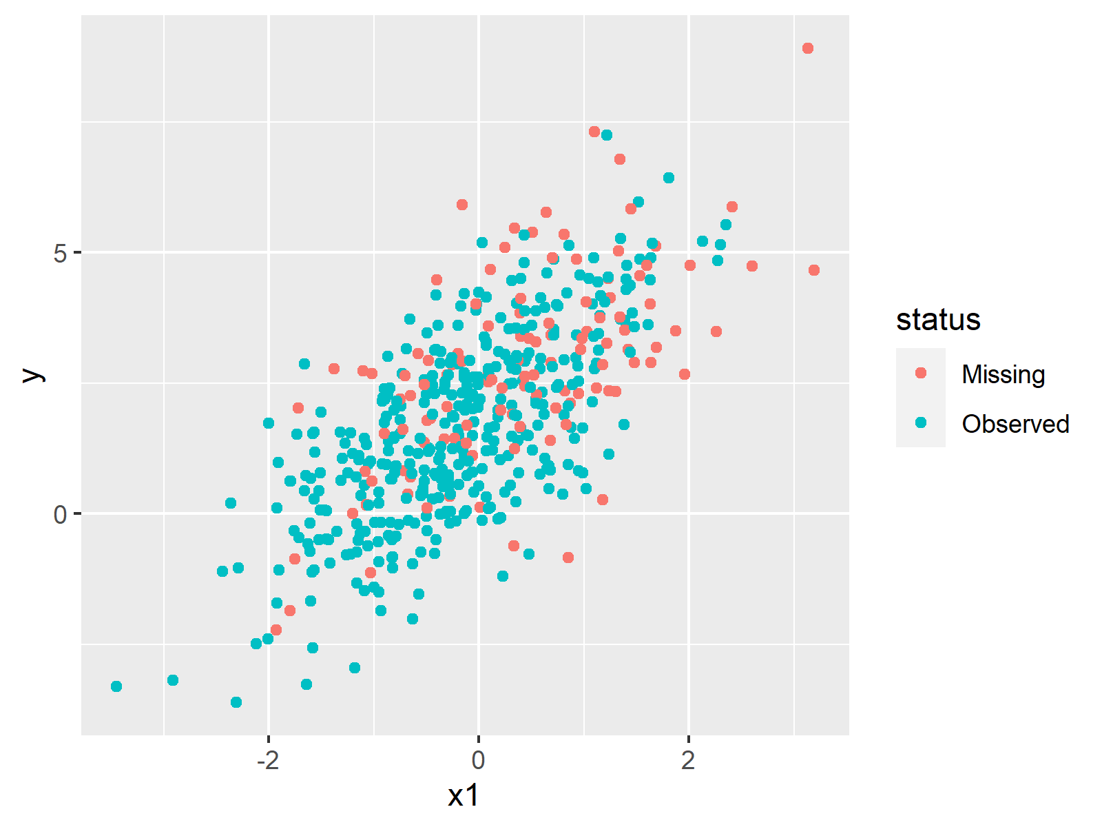
As shown in Figure 1, the previous syntax has created a scatterplot containing the values of y and x1. The observed values are shown in green and the true (but missing) values are shown in red.

This visualization also shows that our missing values follow a pattern, i.e. the higher the values in x1, the more likely it is that a missing value occurs in y. In other words: there are more red dots on the right side of the plot.

Such patterns can be described based on so-called response mechanisms. In our case, the response mechanism is MAR (Missing At Random). You can learn more about the different response mechanisms here.

So far so good, but how can we replace those NA values with estimated imputed values? That’s what I’m going to show you next!

So far so good, but how can we replace those NA values with estimated imputed values? That’s what I’m going to show you next!

Impute Missing Values Using Predictive Mean Matching

This section shows how to substitute the missing values in our data using the predictive mean matching method.

For this, we first have to install and load the mice package to R:

install.packages(""mice"")                                      # Install & load mice
library(""mice"")

In the next step, we can apply the complete() and mice() functions to impute our data. By specifying the method argument to be equal to “pmm”, we tell mice to impute based on the predictive mean matching method.

Note that we are using a single imputation to impute our data. This simplifies our result and allows us to analyze the output with less complexity. However, in real applications multiple imputation is highly recommended, because otherwise the variance estimates of your analysis may be biased.

Anyway, let’s impute our data!

data_imp <- complete(mice(data,                                 # Predictive mean matching imputation
                          m = 1,
                          method = "pmm"))

The previous R code has created a complete data set without missing values called data_imp. Let’s have a look at the first six rows of our imputed data:

head(data_imp)                                                  # Head of imputed data
#      y    x1   x2   x3
# 1 1.85  0.18 0.14 4.47
# 2 4.90  1.63 0.92 6.48
# 3 2.38  0.40 0.49 5.38
# 4 3.22  0.07 0.24 4.55
# 5 1.15 -0.58 0.48 2.39
# 6 0.42 -0.05 0.32 1.60

Remember that the second and third row of our input data frame were missing in the variable y? As you can see, this is not the case in our imputed data. We have filled new values into the missing cells!

Looks good, but this has to be done with care! If missing data imputation is done the wrong way, we may even introduce bias to our data.

Since we are working with synthetic data that we have created ourselves, we can easily investigate how well the imputation process worked. First, we have to create a new data frame with all relevant data, i.e. the true (but missing) values and the imputed values:

data_true_imp <- data.frame(                                    # Data with true & imputed values
  Missing = data_true[data_true$status == ""Missing"", ""y""],
  Imputed = data_imp[data_true$status == ""Missing"", ""y""])

If the correlation between our true and imputed values is high, we can tell that the imputation worked well. To visualize this correlation, we can draw another ggplot2 scatterplot, in which we are plotting the true vs. the imputed values:

ggplot(data_true_imp,                                           # Draw true vs. imputed values
       aes(x = Missing,
           y = Imputed)) +
  geom_point() +
  geom_smooth(method = ""lm"",
              formula = y ~ x)

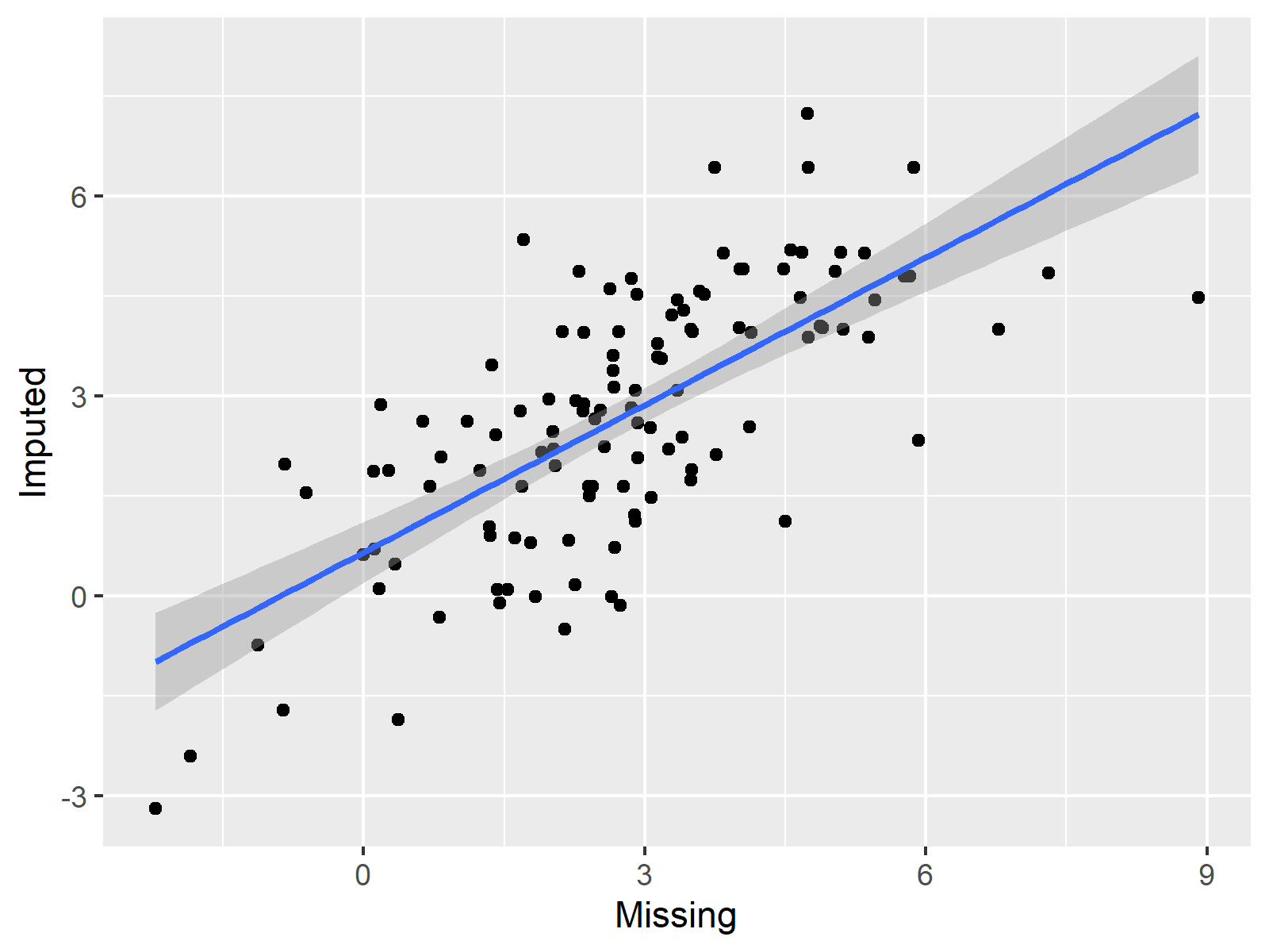
As you can see, the correlation shown in the previous scatterplot is fairly high. Looks good!

Unfortunately, we are not able to make such an evaluation in real life examples, since we do not know the true values of our missing data. For that reason, it is very important to make sure that the imputation model and the imputation method is selected wisely.

In case you may want to learn more about NA values in R, I recommend watching the following video on the Statistics Globe YouTube channel. The video does not explain missing data imputation techniques. However, the video shows some additional functions that may help to handle the missing values in your data!

https://www.youtube.com/watch?v=q8eR2suCyGk

About the Author

This article has been written by Joachim Schork. Joachim is a statistician, R programmer, and the founder of the Statistics Globe education platform. You can find more tutorials of Joachim by visiting his homepage https://statisticsglobe.com/ or his YouTube channel https://www.youtube.com/c/statisticsglobe.

Social media links for the Colaboradores page: https://twitter.com/JoachimSchork https://www.linkedin.com/company/75547611/admin/ https://www.facebook.com/statisticsglobecom/