Recreating the momentum factor (WML) with Brazilian stocks (in R)

Recreating the momentum factor (WML) with Brazilian stocks (in R) published at the "Open Code Community"

Financial literature has been developing and testing factors that help explain the cross section of stock returns for a long time. In a nutshell, the momentum factor (also known as winners minus losers WML) is the tendency for rising asset prices to continue rising, as well as falling prices to continue falling. The WML factor was firstly studied by Jagadeesh and Titman (1993) and Carhart (1997).

This is one of the several factors that help explain asset returns. Factor investing has been gaining grounds in the Brazilian market. Many quantitative mutual funds use a myriad of factors and systematic trading strategies trying to generate alpha and manage risk for their portfolios.

In this post, let’s recriate the momentum factor for stocks listed at the B3 exchange (Brazil) using R. The idea is to create a portfolio that is long in stocks with rising prices and short in stocks with falling prices given a time period. This is pretty simple, however handling the data before creating long and short portfolios may be tricky. That is why I have written this post: if you get the hang of it, it is possible to replicate, or create, any other factor. Whether your are an academic or a practitioner, it may be helpful. In my opinion, after reading many academic papers about portfolio construction sometimes it is not clear how the authors code the many filters used to construct the factors. So, I hope this post help others that may have the same thoughts.

As a guide to construct the WML factor, we will use the NEFIN-USP methodology page. First, let’s clear our workspace and load the required packages. Two special notes: 1) the new version of the ‘BatchGetSymbols’ package of Marcelo Perlin has a nice function to go parallel in fetching financial data. 2) The ‘nefindata’ allows us to get NEFIN-USP data. The package has already been used in this post. Also, our code imports a list of tickers containing active and inactive tickers for companies listed in B3 (former BM&FBovespa). These tickers were gathered at Economatica.

    rm(list=ls()) ### clear workspace, memory and close open plots
    gc()
    graphics.off()

    library(plyr) # data handling
    library(lubridate)
    library(readr) # data reading
    library(BatchGetSymbols) #fetching financial data
    library(future) #parallel computing
    library(zoo)
    library(tidyquant) #financial data handling
    library(reshape2)
    library(ggplot2)

    if (!require('nefindata')) devtools::install_github('fernandoramacciotti/nefindata/R-package')

    tickers <- read.csv('https://www.dropbox.com/s/4cj90vxwbdn3tab/tickers.txt?dl=1') #tickers file
    tickers <- paste(tickers$ticker,'.SA',sep='') # All Yahoo Finance tickers include .SA at the end of the ticker. 
    tickers <- c(tickers,'^BVSP') # Include benchmark

Now we download historical adjusted prices, format dates and calculate financial volume. As we want monthly data on the momentum factor, the yearmon variable is important to be defined. As it may take a while to download historical prices, I suggest to go parallel.

    first.date <- '2011-01-01'
    last.date <- '2021-05-30'
    freq <- 'daily' 

    future::plan(future::multisession, # Enables parallel computing
             workers = 3) # Define number of cores

	
    raw.df <- BatchGetSymbols(tickers = tickers,first.date = first.date  #Fetching data from Yahoo Finance
                      ,last.date = last.date
                      ,type.return = 'log'
                      ,freq.data = freq
                      ,thresh.bad.data = 0.01 # we will filter data frequency later
                      ,bench.ticker = '^BVSP'
                      ,do.parallel = TRUE #disable if you don't want to go parallel
                      )

	
    df <- raw.df$df.tickers
    df <- df %>% mutate(ticker= gsub(pattern = '\\^',replacement = '',x = ticker) #remove the '^' from ^BVSP ticker
                    ,sticker= substr(ticker,1,4) #Retrieve short tickers to filter same-company asset codes,
                    ,year=year(ref.date)
                    ,month=month(ref.date)
                    ,fvolume=volume*df$price.close #Yahoo data provides the  number of shares traded, not financial volume.
                    ,yearmon=as.yearmon(ref.date)
                    ,tickeryear=paste(ticker,year,sep='')
                    )

According to NEFIN, a stock is eligible to the sample if it meets three criteria:

1. The stock is the most traded stock of the firm (the one with the highest traded volume during last year).

    df.vol <- df %>% group_by(ticker,sticker,year) %>%
        summarize(svol=sum(fvolume),count=n()) %>% 
        mutate(lvol=lag(svol,1,order_by = year),lcount=lag(count,1,order_by = year))
   
    df.vol$tickeryear=paste(df.vol$ticker,df.vol$year,sep='')
    df1 <- df.vol %>% group_by(sticker,year) %>% top_n(1,lvol) # pick the most traded asset if there is more than one ticker for a given company.
   

2. The stock was traded in more than 80% of the days in year t-1 with volume greater than R$ 500.000,00 per day. In case the stock was listed in year t-1, the period considered goes from the listing day to the last day of the year.

    thresh <- 0.8
    volume <- 500000
   
    df$ptrade <- df$fvolume > volume
   
    df2 <- df %>% group_by(ticker,year) %>% 
        summarise(nthresh=sum(ptrade)) %>% mutate(nthreshl=lag(nthresh,1))
   
    df2 <-join(x=df2,y=df.vol,by=c('ticker','year')) %>% 
        mutate(pthresh=nthresh/count, pthreshl=nthreshl/lcount) %>%
        filter(pthreshl>thresh)
   

3. The stock was initially listed prior to December of year t-1.

As the listing date is not available, we will consider whether data is available at year t-1 (spoiler: this will cause a small diference between our results and NEFIN’s).

    df3 <- df %>%
        group_by(ticker) %>%
        mutate(first_year = min(year)) %>%
        filter(year > first_year) %>%
        select(-c(first_year))

Now that we have the stocks eligible for each criteria, we collapse them to find unique stock-year observations.

    ftickers <- Reduce(intersect,list(df1$tickeryear,df2$tickeryear,df3$tickeryear))

Some of the eligibility criteria are based on daily data, eventhough we need monthly data to calculate portfolios. The following of code calculates monthly returns:

        port <- df %>% group_by(ticker) %>% tq_transmute(select = 'price.adjusted'
                                                ,mutate_fun = periodReturn
                                                ,period='monthly'
                                                ,type = 'log'
                                                ,leading=FALSE) 
      
    port<- port %>% rename(mret = monthly.returns)
    port$yearmon <- as.yearmon(port$ref.date)
    closing.prices <- df %>% select(c(ticker,ref.date,price.adjusted))
  
    nport <- join(x = port,y = closing.prices,by = c('ticker','ref.date'))

It is time to create the long and short portfolios. Quoting from the Nefin website: ‘Every month t, we (ascending) sort the eligible stocks (as defined in Section 2) in terciles according to their cumulative returns from month t-12 and month t-2. We then hold the portfolios during month t’. Thus, we need to calculate t-12 and t-2 returns. Note that until now we had the full sample of returns. It is time to keep only eligible stocks.

    ndf <- nport %>% 
        arrange(ref.date) %>% group_by(ticker) %>% 
        mutate(lret=log(lag(price.adjusted,2)/lag(price.adjusted,12)))

    ndf$year<- year(ndf$ref.date)
    ndf$tickeryear <- paste(ndf$ticker,ndf$year,sep='')
    ndf <- ndf %>% filter (tickeryear %in% ftickers) #keep only eligible stocks

Now we classify stocks by terciles, create the long and short portfolios and calculate the cumulative returns of the portfolio.

    ndf <- ndf %>% group_by(yearmon) %>% 
        mutate(tercile=ntile(x = lret,n = 3))

    wml <- na.omit(ndf) %>% group_by(yearmon) %>% 
        summarise(wml=mean(mret[tercile==3])-mean(mret[tercile==1])) %>% ungroup() %>% mutate(cwml=cumprod(1+wml))

Voilà! Our momentum factor is created. Now let’s compare it to the actual NEFIN data. As we don’t have the listing date of a company, note that the third eligibility criteria is quite different than the original. Also, the initial tickers may be distinct between this code and the one used by NEFIN.

    nefin <- get_risk_factors(factors = 'WML',agg = 'daily')
    nefin <- nefin %>% mutate(ref.date=as.Date(paste(year,'-',month,'-',day,sep = '')))
    nefin$yearmon <- as.yearmon(nefin$ref.date)

    nefin <- nefin %>% arrange(ref.date) %>%
          group_by(yearmon) %>% summarise(nefin_wml=(prod(1+WML)-1))


    fdf <- join(x = wml,y = nefin,by='yearmon') %>% # Merging our data with NEFIN's
        mutate(cnefin_wml=cumprod(1+nefin_wml))

    print(cor(fdf$wml,fdf$nefin_wml))

The correlation between data is pretty decent (0.9447842). Let’s plot the cumulative return of $1 invested in the strategy:

    ldf <- melt(data = fdf,id.vars = 'yearmon') # long format for ggplot
    p <- ggplot(filter(ldf,variable %in% c('cwml','cnefin_wml'))) + geom_line(aes(y=value,x=yearmon,group=variable,color=variable))
    p<- p + xlab(label = 'Date') + ylab(label='Cumulative return')
    print(p)

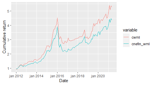
How about that? The rationale of developing the momentum factor is similar to other (older) factors such as Small minus Big (SMB) or High minus Low (HML). As financial markets develop, new factors that affect asset pricing are uncovered by acadmemics and practitioners. There are many factors developed by financial literature that have not been tested in the Brazilian market (at least not academically). In this post we used past returns to build a factor, but one could use other aspects such as beta, downside, liquidity, size, firm characteristics and etc.

Suggestions for improving the code or comments at general are more than welcome at email or at LinkedIn.

References

CARHART, Mark M. On persistence in mutual fund performance. The Journal of finance, v. 52, n. 1, p. 57-82, 1997.

JEGADEESH, Narasimhan; TITMAN, Sheridan. Returns to buying winners and selling losers: Implications for stock market efficiency