Testing static asset allocations
Simple Buy-and-Hold Asset Allocations
In this Markdown, I test 16 simple ``buy-and-hold'' asset allocation strategies using ETF data. This post was inspired by a thread on Twitter which provided descriptions and some performance stats for these constant allocation portfolios.1 The allocations are the following (ETF names/asset classes are provided at the end):
Golden Butterfly: SHY(20%), TLT (20%), VTI (20%), IWN (20%), GLD (20%)
Rob Arnott Portfolio: BNDX (20%), LQD (20%), VEU (10%), VNQ (10%), SPY (10%), TLT (10%), TIP (10%), DBC(10%)
Global Asset Allocation Portfolio: SPY (18%), EFA (13.5%) , EEM (4.5%) , LQD (19.8%) , BNDX (14.4%) , TLT (13.5%) , TIP (1.8%) , DBC (5%) , GLD (5%) , VNQ (4.5% )
Permanent Portfolio: BIL (25%), GLD(25%), TLT (25%), SPY (25%)
Desert Portfolio: IEF (60%), VTI(30%), GLD(10%)
The Larry Portfolio: IWN (15%), DLS (7.5%), EEM (7.5%), IEF (70%)
Big Rocks Portfolio: AGG (60%), SPY (6%), IWD (6%), IWM (6%), IWN (6%), EFV (4%), VNQ (4%), EFA (2%), SCZ (2%), DLS (2%), EEM (2%)
Sandwich Portfolio: IEF (41%), SPY (20%), SCZ (10%), IWM (8%), EEM (6%), EFA (6%), VNQ (5%), BIL (4%)
Balanced - Tax Aware Portfolio: AGG (38%), SPY (15%), BIL (15%), EFA (13%), IWM (5%), VNQ (5%), DBC (5%), EEM (4%)
Balanced Portfolio: AGG (33%), SPY (15%), BIL (15%), EFA (13%), IWM (5%), VNQ (5%), DBC (5%), EEM (4%), TIP (2%), BNDX (2%), HYG (1%)
Income With Growth Portfolio: AGG (37%), BIL (20%), TIP (10%), SPY (9%), EFA (8%), VNQ (5%), HYG (4%), BNDX (4%), IWM (2%), DBC (1%)
Income Growth Tax Portfolio: AGG (55%), BIL (20%), SPY (9%), EFA (8%), VNQ (5%), IWM (2%), DBC (1%)
Conservative Income Portfolio: AGG (40%), BIL (25%), TIP (18%), HYG (7%), VNQ (5%), BNDX (5%)
Conservative Income Tax Portfolio: AGG (70%), BIL (25%), VNQ (5%)
All Weather Portfolio: SPY (30%), TLT (40%), IEF (15%), GLD (7.5%), DBC (7.5%)
United Stated 60/40 Portfolio: SPY (60%), IEF (40%)
These portfolios are simple to implement, as they involve only a few ETFs. However they require rebalancing to maintain the desired allocations. I assume rebalancing is done at the end of each month to facilitate the calculation of returns. I do not consider transaction costs.
Representing each strategy
The first step is to create an object with each strategy. I use a simple list with the tickers and weights:
# create each allocation strategy as a list of tickers and weights
golden_butterfly <- list(tickers = c("SHY", "TLT", "VTI", "IWN", "GLD"),
                        weights = c(0.20, 0.20, 0.20, 0.20, 0.20))

rob_arnott <- list(tickers = c("BNDX", "LQD", "VEU", "VNQ", "VNQ", "SPY", "TLT", "TIP", "DBC"),
                   weights = c(0.20, 0.20, 0.10, 0.10, 0.10, 0.10, 0.10, 0.10, 0.10))

globalAA <- list(tickers = c("SPY", "EFA", "EEM", "LQD", "BNDX", "TLT", "TIP", "DBC", "GLD", "VNQ"),
                 weights = c(0.18, 0.135, 0.045, 0.18, 0.144, 0.135, 0.018, 0.05, 0.05, 0.045))

permanent <- list(tickers = c("BIL", "GLD", "TLT", "SPY"),
                  weights = c(0.25, 0.25, 0.25, 0.25))

desert <- list(tickers = c("IEF", "VTI", "GLD"),
               weights = c(0.60, 0.30, 0.10))

larry <- list(tickers = c("IWN", "DLS", "EEM", "IEF"),
              weights = c(0.15, 0.075, 0.075, 0.70))

big_rocks <- list(tickers = c("AGG", "SPY", "IWD", "IWM", "IWN", "EFV", "VNQ", "EFA", "SCZ", "DLS", "EEM"),
                  weights = c(0.60, 0.06, 0.06, 0.06, 0.06, 0.04,0.04, 0.02, 0.02, 0.02, 0.02))

sandwich <- list(tickers = c("IEF", "SPY", "SCZ", "IWM", "EEM", "EFA", "VNQ", "BIL"),
                  weights = c(0.41, 0.20, 0.10, 0.08, 0.06, 0.06, 0.05, 0.04))


balanced_tax <- list(tickers = c("AGG", "SPY", "BIL", "EFA", "IWM", "VNQ", "DBC", "EEM" ),
                           weights = c(0.38, 0.15, 0.15, 0.13, 0.05, 0.05, 0.05, 0.04))

balanced <- list(tickers = c("AGG", "SPY", "BIL", "EFA", "IWM", "VNQ", "DBC", "EEM", "TIP", "BNDX", "HYG"),
                 weights = c(0.33, 0.15, 0.15, 0.13, 0.05, 0.05, 0.05, 0.04, 0.02, 0.02, 0.01))

income_gr <- list(tickers = c("AGG", "BIL", "TIP", "SPY", "EFA", "VNQ", "HYG", "BNDX", "IWM", "DBC"),
                      weights = c(0.37, 0.20, 0.10, 0.09, 0.08, 0.05, 0.04, 0.04, 0.02, 0.01))

income_gr_tax <- list(tickers = c("AGG", "BIL", "SPY", "EFA", "VNQ", "IWM", "DBC"),
                          weights = c(0.55, 0.20, 0.09, 0.08, 0.05, 0.02, 0.01))

con_income  <- list(tickers = c("AGG", "BIL", "TIP", "HYG", "VNQ", "BNDX"),
                             weights = c(0.40, 0.25, 0.18, 0.07, 0.05, 0.05))

con_income_tax  <- list(tickers = c("AGG", "BIL", "VNQ"),
                    weights = c(0.70, 0.25, 0.05))

all_weather  <- list(tickers = c("SPY", "TLT", "IEF", "GLD", "DBC"),
                     weights = c(0.30, 0.40, 0.15, 0.075, 0.075))

us_60_40 <- list(tickers = c("SPY", "IEF"),
                  weights = c(0.60, 0.40))
Retrieving the data
To download the data, I use the getSymbols function from the quantmod package. I also load the PerformanceAnalytics package, which makes calculation of performance metrics trivial. I keep only end-of-month data and then calculate the monthly returns of all ETFs. I also download the yield on the 3-month T-bill from FRED and align it with the ETF data.
library(quantmod)
library(PerformanceAnalytics)

# get all the unique tickers
tickers <- unique(c(golden_butterfly$tickers,
                    rob_arnott$tickers,
                    globalAA$tickers,
                    permanent$tickers,
                    desert$tickers,
                    larry$tickers,
                    big_rocks$tickers,
                    sandwich$tickers,
                    balanced_tax$tickers,
                    balanced$tickers,
                    income_gr$tickers,
                    income_gr_tax$tickers,
                    con_income$tickers,
                    all_weather$tickers,
                    us_60_40$tickers))

# download prices for all tickers from Yahoo Finance
getSymbols(tickers, from = "2007-06-01", source = 'yahoo')
##  [1] "SHY"  "TLT"  "VTI"  "IWN"  "GLD"  "BNDX" "LQD"  "VEU"  "VNQ"  "SPY"
## [11] "TIP"  "DBC"  "EFA"  "EEM"  "BIL"  "IEF"  "DLS"  "AGG"  "IWD"  "IWM"
## [21] "EFV"  "SCZ"  "HYG"
# align all prices into one xts object
prices <- xts()
for (i in 1:length(tickers)){
  prices  <- merge.xts(prices, get(tickers[i])[,6])
}
colnames(prices) <- tickers

# keep only month ends - could do it daily but who's got time?
prices <- prices[endpoints(prices, on = "months"),]

#calculate returns
returns <- CalculateReturns(prices)

# download risk-free (3-month Tbill from FRED) and align with monthly frequency
getSymbols("DGS3MO", src = "FRED")
## [1] "DGS3MO"
tbill <- DGS3MO[index(returns)]/100/12
Calculating the returns of each strategy
I create a function to calculate the returns of each allocation strategy. Since the portfolios are rebalanced on a monthly basis, the monthly returns can be obtained simply by multiplying the weights by the corresponding ETF returns. I start calculation of returns from the date when all ETF returns are available.
calculate_strat_returns <- function(strat, returns){

  dates <- index(returns)

  # convention: start the backtest when data for all assets is available
  returns_strat <- returns[, strat$tickers]
  first_index <- which.max((!is.na(rowSums(returns_strat))))

  n_assets <- length(strat$tickers)
  weights <- rbind(matrix(NA, nrow = first_index - 1, ncol = n_assets),
                   matrix(strat$weights, nrow = nrow(returns) - first_index + 1,
                          ncol = n_assets, byrow = TRUE))

  strat_returns <- xts(rowSums(weights * returns_strat), order.by = index(returns))
  return(strat_returns)
}
I then loop through each strategy and calculate their returns:
strats <- c("golden_butterfly",
            "rob_arnott",
            "globalAA",
            "permanent",
            "desert",
            "larry",
            "big_rocks",
            "sandwich",
            "balanced_tax",
            "balanced",
            "income_gr",
            "income_gr_tax",
            "con_income",
            "con_income_tax",
            "all_weather",
            "us_60_40")

# calculate returns of all strategies
strat_returns <- xts()
for (i in 1:length(strats)){
  this_strat <- calculate_strat_returns(get(strats[i]), returns)
  strat_returns <- merge.xts(strat_returns,
                             this_strat)
}
colnames(strat_returns) <- strats
Performance of different strategies
Now I can calculate some performance metrics using functions from PerformanceAnalytics and display the results in a table. The annualized returns range from 2.63% for the Conservative Income strategy to 8.15% for the United Stated 60/40 strategy. The Desert portfolio produces the highest Sharpe ratio (1.04), while the Sandwich portfolio produces the lowest (0.33).
# calculate some statistics
table1 <- table.AnnualizedReturns(strat_returns, Rf = tbill)
table2 <- table.DownsideRiskRatio(strat_returns, MAR = mean(tbill))
table3 <- table.DownsideRisk(strat_returns, Rf = mean(tbill))

table_metrics <- rbind(table1,
                       table2[c("Annualised downside risk",
                                "Sortino ratio"), ],
                       table3[c("Historical VaR (95%)",
                                "Historical ES (95%)",
                                "Maximum Drawdown"),])

library(kableExtra)
kbl(t(table_metrics), caption =  "Performance metrics for buy & hold asset allocation strategies") %>%
  kable_classic()
| Annualized Return | Annualized Std Dev | Annualized Sharpe (Rf=0.68%) | Annualised downside risk | Sortino ratio | Historical VaR (95%) | Historical ES (95%) | Maximum Drawdown | |
|---|---|---|---|---|---|---|---|---|
| golden_butterfly | 0.0721 | 0.0795 | 0.8194 | 0.0507 | 0.3774 | -0.0289 | -0.0503 | 0.1663 |
| rob_arnott | 0.0664 | 0.0761 | 0.7777 | 0.0493 | 0.3548 | -0.0302 | -0.0443 | 0.1194 |
| globalAA | 0.0652 | 0.0677 | 0.8578 | 0.0417 | 0.4069 | -0.0266 | -0.0379 | 0.0930 |
| permanent | 0.0661 | 0.0689 | 0.8604 | 0.0404 | 0.4269 | -0.0246 | -0.0371 | 0.1280 |
| desert | 0.0678 | 0.0589 | 1.0337 | 0.0358 | 0.4890 | -0.0207 | -0.0346 | 0.1113 |
| larry | 0.0507 | 0.0601 | 0.7305 | 0.0398 | 0.3232 | -0.0254 | -0.0393 | 0.1295 |
| big_rocks | 0.0520 | 0.0769 | 0.6032 | 0.0526 | 0.2577 | -0.0298 | -0.0526 | 0.2249 |
| sandwich | 0.0609 | 0.0916 | 0.6025 | 0.0627 | 0.2612 | -0.0383 | -0.0623 | 0.2895 |
| balanced_tax | 0.0463 | 0.0801 | 0.4934 | 0.0559 | 0.2161 | -0.0347 | -0.0558 | 0.2704 |
| balanced | 0.0547 | 0.0635 | 0.7504 | 0.0414 | 0.3393 | -0.0251 | -0.0373 | 0.1062 |
| income_gr | 0.0424 | 0.0413 | 0.8564 | 0.0262 | 0.3927 | -0.0149 | -0.0238 | 0.0586 |
| income_gr_tax | 0.0402 | 0.0494 | 0.6790 | 0.0330 | 0.2973 | -0.0181 | -0.0332 | 0.1437 |
| con_income | 0.0263 | 0.0283 | 0.6861 | 0.0176 | 0.3220 | -0.0109 | -0.0155 | 0.0375 |
| con_income_tax | 0.0313 | 0.0324 | 0.7605 | 0.0194 | 0.3664 | -0.0113 | -0.0186 | 0.0468 |
| all_weather | 0.0740 | 0.0742 | 0.9036 | 0.0472 | 0.4138 | -0.0286 | -0.0451 | 0.1363 |
| us_60_40 | 0.0806 | 0.0885 | 0.8317 | 0.0576 | 0.3754 | -0.0370 | -0.0580 | 0.2946 |
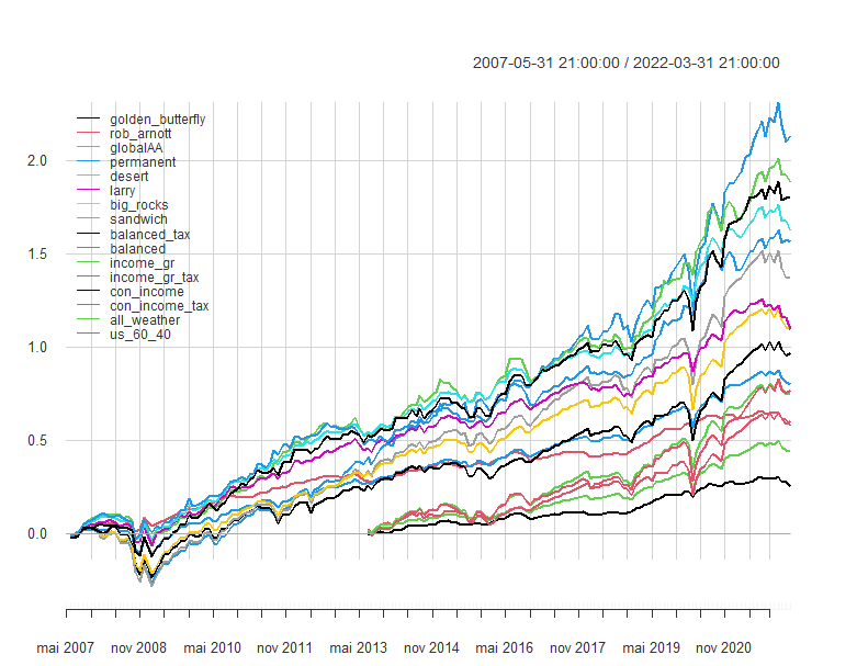
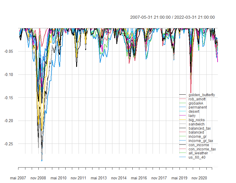
Next I plot the cumulative returns and drawdowns of the strategies. The drawdowns in 2007-2008 for most strategies are in the 10-20% range. The United Stated 60/40, which is considered by many as a good constant allocation benchmark, produces the highest drawdown at 29.5%.
# plot cumulative returns
chart.CumReturns(strat_returns,
                 begin = "axis",
                 legend.loc = "topleft")
# drawdowns
chart.Drawdown(strat_returns,
               legend.loc = "bottomright")
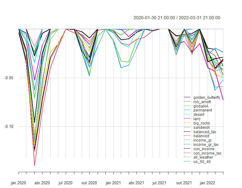
Finally, I zoom in on the recent period starting in 2020. Most strategies lose up to 10% during the first months of 2020 as the pandemic hits. Since most strategies have sizable allocations to bonds, it’s not surprising to see how they have all suffered since the end of 2021, as rates start to increase.
# plot cumulative returns
chart.CumReturns(strat_returns["2020/"],
                 begin = "axis",
                 legend.loc = "topleft")
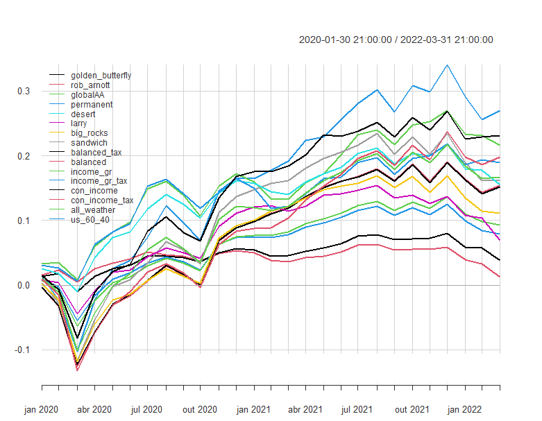
chart.Drawdown(strat_returns["2020/"],
               legend.loc = "bottomright")
Conclusion
In this short R Markdown, I calculate returns and performance metrics of 16 popular static asset allocation strategies. These strategies are simple to implement using ETFs, and several of them have produced very decent risk-adjusted returns in the past. The million-dollar question is, what kind of allocation will perform well in the current (and unprecedented) environment?
Some interesting extensions: calculate returns on a daily basis and also for tactical asset allocation schemes, such as the Ivy portfolio.
List of ETFs
| TICKER | Fund Name | Fund Type | Geographic Focus |
| AGG | iShares Core US Aggregate Bond ETF | Bond | United States of America |
| BIL | SPDR Bloomberg 1-3 Month T-Bill ETF | Bond | United States of America |
| BNDX | Vanguard Total International Bond Index Fund;ETF | Bond | Global Ex US |
| DBC | Invesco DB Commodity Index Tracking Fund | Commodity | United States of America |
| DLS | WisdomTree International SmallCap Dividend Fund | Equity | Global Ex US |
| EEM | iShares MSCI Emerging Markets ETF | Equity | Global Emerging Markets |
| EFA | iShares MSCI EAFE ETF | Equity | Global Ex US |
| EFV | iShares MSCI EAFE Value ETF | Equity | Global Ex US |
| GLD | SPDR Gold Shares | Commodity | Global |
| HYG | iShares iBoxx $ High Yield Corporate Bond ETF | Bond | United States of America |
| IEF | iShares 7-10 Year Treasury Bond ETF | Bond | United States of America |
| IWD | iShares Russell 1000 Value ETF | Equity | United States of America |
| IWM | iShares Russell 2000 ETF | Equity | United States of America |
| IWN | iShares Russell 2000 Value ETF | Equity | United States of America |
| LQD | iShares iBoxx $ Inv Grade Corporate Bond ETF | Bond | United States of America |
| SCZ | iShares MSCI EAFE Small-Cap ETF | Equity | Global Ex US |
| SHY | iShares 1-3 Year Treasury Bond ETF | Bond | United States of America |
| SPY | SPDR S&P 500 ETF Trust | Equity | United States of America |
| TIP | iShares TIPS Bond ETF | Bond | United States of America |
| TLT | iShares 20+ Year Treasury Bond ETF | Bond | United States of America |
| VEU | Vanguard FTSE All-World ex US Index Fund;ETF | Equity | Global Ex US |
| VNQ | Vanguard Real Estate Index Fund;ETF | Equity | United States of America |
| VTI | Vanguard Total Stock Market Index Fund;ETF | Equity | United States of America |
The thread was posted by @WifeyAlpha which is currently a locked account. ↩︎